Exploring global Land Cover available through the Climate Data Store (CDS)

This notebook can be run on free online platforms, such as Binder, Kaggle and Colab, or they can be accessed from GitHub. The links to run this notebook in these environments are provided here, but please note they are not supported by ECMWF.

Introduction

Land cover is the observed bio-physical cover on the Earth’s surface (Townshend et al., 2008). It is not to be confounded with land use. Land use characterizes the arrangements, socio-economic activities and inputs people are undertaking on a certain land cover type. Land cover regulates energy, water, and carbon cycles, reflects climate change impacts, and provides important information for climate monitoring, modelling, and policy.

Learning objectives 🎯

At the end of this notebook, the user will be able to:

• Understand and use key terminology;

• Retrieve landcover data from the C3S Climate Data Store, examining, subsetting, saving and re-projecting it using Python code;

• Explore landcover change over time;

• Explore landcover regional statistics.

Key Terms

Land Cover (LC) and land cover change (LCC) are becoming increasingly related to the climate modelling effort. Land cover change is a pressing environmental issue acting as both a cause and a consequence of climate change. The importance of these issues requires continuous monitoring systems and the most accurate data. The Copernicus Climate Change Service provides Intermediate Climate Data Records for many Essential Climate Variables, including LC. The global C3S LC maps 2016 – 2022 are, and will remain, consistent with the existing European Space Agency Climate Change Initiative global annual LC maps from 1992 – 2015.

The proposed land cover ontology assumes that the land cover is organized along a continuum of temporal and spatial scales and that each land cover type is defined by a characteristic scale, i.e. by the typical spatial extent and period over which its physical traits are observed (Miller, 1994). This twofold assumption requires introducing the time dimension in the land cover characterization to allow distinguishing between the stable and the dynamic components of the land surface.

The stable component, named “land cover”, refers to the set of land surface features which remain stable over time and thus define the land cover independently of any sources of temporary or natural variability. Conversely, the dynamic component is directly related to this temporary or natural variability that can induce some variation in land surface features over time but without changing the land cover in its essence. This dynamic component is referred to as “land surface seasonality” (Lamarche et al., 2014).

Land cover

In this context, ‘LC change’ (LCC) is therefore considered as a permanent modification of the LC – and not of its conditions – in comparison with a baseline status.

Land cover classes

A LC class refers to a LC category described by a stable ensemble of land surface features forming a LC class (e.g., forest, cropland). Land surface features consist of landscape elementary units (e.g., a house, a tree, a water body, etc.) described by:

1. the type of the observed features, such as tree, shrub, herbaceous vegetation, moss/lichen vegetation, terrestrial or aquatic vegetation, inland water, built-up areas, permanent snow/ice, etc;

2. the structure of the observed features, like the vegetation height, vegetation cover, building density, etc;

3. the nature of the observed features, such as the level of artificiality or some species information (e.g., C3/C4 distinction);

4. the homogeneity of the observed features at the level of observation, leading to pure or mosaic classes. The LC classes are well-defined and described using the UN/FAO Land Cover Classification System (LCCS) (di Gregorio and Jansen, 2005).

Figure 1: Land Cover map including the legend.

References:

• Townshend J. R., Latham J., Arino O., Balstad R., Belward A., Conant R., Elvidge C., Feuquay J., El Hadani D., Herold M., Janetos A., Justice C.O., Liu J., Loveland T., Nachtergaele F., Ojima,D., Maiden M., Palazzo F., Schmullius C., Sessa R., Singh A., Tschirley J. and Yahamoto H., 2008, Integrated Global Observations of the Land: an IGOS-P theme. IGOL Report No. 8, GTOS, 54. Available at: http://www.fao.org/docrep/011/i0536e/i0536e00.htm

• Miller R.I., 1994, Mapping the diversity of the nature, London, New York: Chapman & Hall

• Lamarche, C., Bontemps, S., Rousseau, C., De Maet, T., Verhegghen, A., Radoux, J., Van Bogaert, E., Arino, O. and Defourny, P., 2014. “ CCI-LC seasonality product. Characterizing the reference dynamics of the land surface. In The 4th International Symposium on Recent Advances in Quantitative Remote Sensing: RAQRS’IV.

• Di Gregorio, A. and Louisa J M Jansen (2005). Land Cover Classification. System Classification concepts and user manual. V2.0. (R. Food & Agriculture Organization of the United Nations, Ed.) https://www.fao.org/3/y7220e/y7220e00.htm.

Prepare your environment

The first thing we need to do, is make sure you are ready to run the code while working through this notebook. There are some simple steps you need to do to get yourself set up.

Set up CDSAPI and your credentials

The code below will ensure that the cdsapi package is installed. If you have not setup your ~/.cdsapirc file with your credenials, you can replace None with your credentials that can be found on the how to api page (you will need to log in to see your credentials).

!pip install -q cdsapi
# If you have already setup your .cdsapirc file you can leave this as None
cdsapi_key = None
cdsapi_url = None

[notice] A new release of pip is available: 25.1.1 -> 25.2
[notice] To update, run: python.exe -m pip install --upgrade pip

(Install and) Import libraries

Module name	Description
numpy	NumPy is the fundamental package for scientific computing with Python and for managing ND-arrays.
rasterio	Rasterio is a library that allows operations on gridded raster data such as satellite images or terrain models.
xarray	Xarray is a very user friendly library to manipulate NetCDF files within Python. It introduces labels in the form of dimensions, coordinates and attributes on top of raw NumPy-like arrays, which allows for a more intuitive, more concise, and less error-prone developer experience.
matplotlib	Matplotlib is a Python 2D plotting library which produces high quality figures.
cartopy	Cartopy is a library for plotting maps and geospatial data analyses in Python.
geopandas	Geopandas is a library that allows spatial operation on geometric data.
pandas	Pandas is a library that allows data analysis and manipulation.
odc-geo	odc-geo is a library that allows combination of geometry shape classes from shapely with CRS from pyproj.
xhistogram	xhistogram is a library for fast, flexible, label-aware histograms for numpy and xarray.

# Modules system
import os

# Modules related to data retrieving
import earthkit as ek
import cdsapi

# Modules related to plot and EO data manipulation
import numpy as np
import xarray as xr
import matplotlib.pyplot as plt
from matplotlib import colors as mcolors
import cartopy.crs as ccrs
import pandas as pd
import geopandas as gpd

Specify data directory

Below we define a directory to store the files locally, and create this directory if it does not already exist

# Directory to store data
# Please ensure that data_dir is a location where you have write permissions
DATADIR = './data_dir/'
# Create this directory if it doesn't exist
os.makedirs(DATADIR, exist_ok=True)

Explore data

The data used in the examples are the satellite-based Land Cover products that provide global maps describing the land surface into 22 classes defined using the United Nations Food and Agriculture Organization’s (UN FAO) Land Cover Classification System (LCCS).

From the WEkEO Data Viewer, you can explore all the products available with many filters to select the region you are interested in, the parameters you want to study, etc.

The C3S Land Cover dataset provides global maps describing the land surface into the 22 LCCS classes. In addition to the land cover (LC) data, four quality flags are included in the dataset to document the reliability of the classification and change detection.

In order to ensure continuity, these land cover maps are consistent with the series of global annual LC maps from the 1990s to 2015 produced by the European Space Agency (ESA) Climate Change Initiative (CCI), which are also available on the ESA CCI LC viewer.

To produce this dataset, the entire Medium Resolution Imaging Spectrometer (MERIS) Full and Reduced Resolution archive from 2003 to 2012 was first classified into a unique 10-year baseline LC map. This is then back- and up-dated using change detected from (i) Advanced Very-High-Resolution Radiometer (AVHRR) time series from 1992 to 1999, (ii) SPOT-Vegetation (SPOT-VGT) time series from 1998 to 2012 and (iii) PROBA-Vegetation (PROBA-V) and Sentinel-3 OLCI (S3 OLCI) time series from 2013.

Beyond the climate-modelling communities, this dataset’s long-term consistency, yearly updates, and high thematic detail on a global scale have made it attractive for a multitude of applications such as land accounting, forest monitoring and desertification, in addition to scientific research.

DATA	DESCRIPTION
Data type	Gridded
Projection	Plate Carrée
Horizontal coverage	Global
Horizontal resolution	300 m
Vertical coverage	Surface
Vertical resolution	Single level
Temporal coverage	1992 to present with one year delay
Temporal resolution	Yearly
File format	NetCDF4
Conventions	Climate and Forecast (CF) Metadata Convention v1.6 and ESA CCI Data Standards [DSWG 2015]
Versions	Version 2.0.7cds provides the LC maps for the years 1992 – 2015; version 2.1.1 for the years after 2016. Both versions are produced with the same processing chain.
Update frequency	Yearly

	MAIN VARIABLES
Name	Units	Description
Change count	Dimensionless	Number of years where land cover class changes have occurred, since 1992. 0 for stable, greater than 0 for changes.
Current pixel state	Dimensionless	Pixel identification from satellite surface reflectance observations, mainly distinguishing between land, water, and snow/ice. Six values are used: 1, 2, 3, 4, 5, 6; respectively meaning: clear land, clear water, clear snow ice, cloud, cloud shadow, filled.
Land cover class	Dimensionless	Land cover class per pixel, according to a legend of 22 classes, defined using the Land Cover Classification System developed by the United Nations Food and Agriculture Organization. Distinct values are encoded as unsigned byte (0..255). The complete legend is available in the NetCDF files metadata and in the Product User Guide documentation.
Observation count	Dimensionless	Number of valid satellite observations that have contributed to each pixel’s classification
Processed flag	Dimensionless	Flag to mark areas that could not be classified. Two values are used: 0, 1; respectively meaning: not_processed, processed.

You can also visit the Copernicus Climate Data Store pages dedicated to the products (Land cover) to see more detail about the product and all the different variables that are available.

Download the data

There are different ways to download data in ECMWF Climate Data Store. You can do it manually from the Data Download TAB, or you can also download the data using the CDS-API. We write the API request, i.e. specify which product we want, which parameters, etc. To write a new request, the easiest way is to select your data parameters in the CDS, click on Show API request, and copy/paste it in a file (or directly in a notebook cell).

Warning

Please remember to accept the terms and conditions of the dataset, at the bottom of the CDS download form.

First we will connect our cdsapi client:

c = cdsapi.Client(url=cdsapi_url, key=cdsapi_key)

# Define a download filename:
download_filename_2022 = f"{DATADIR}/lc_2022.zip"

# Downloading ba-pixel product over Europe
dataset = "satellite-land-cover"
request = {
    "variable": "all",
    "year": ["2022"],
    "version": ["v2_1_1"]
}

if not os.path.exists(download_filename_2022):
    c.retrieve(dataset, request, download_filename_2022)
else:
    print(f"File {download_filename_2022} already exists. Skipping download.")

lc_data = ek.data.from_source("file", download_filename_2022)
lc_data

2025-09-23 16:51:37,862 INFO [2025-09-03T00:00:00] To improve our C3S service, we need to hear from you! Please complete this very short [survey](https://confluence.ecmwf.int/x/E7uBEQ/). Thank you.
2025-09-23 16:51:37,862 INFO [2024-09-26T00:00:00] Watch our [Forum](https://forum.ecmwf.int/) for Announcements, news and other discussed topics.

File ./data_dir//lc_2022.zip already exists. Skipping download.

NetCDFFieldListReader(C:\Users\Grit\AppData\Local\Temp\tmpkqxyyu5_\file-50addd524ed19cb08ce0fb8486bbcd0f2f80f68b8598433c9317929f6148eb3a.d\C3S-LC-L4-LCCS-Map-300m-P1Y-2022-v2.1.1.nc)

Visualise the C3S & CCI Land Cover dataset

Let’s take a first quick look at the dataset! Let’s plot for example the year 2022 for the regiom Kerala - a southern Indian state known for its backwaters, tropical beaches, tea plantations, and rich culture!

Application main steps:

• Definition of the color map based on the LCCS Legend

• Define a subset based on the latitude and longitude values

• Compose a title

• Show the result on a map using the chosen title

• Save the subset and the image

# Definition of the color map based on the LCCS Legend

cmap = mcolors.ListedColormap([
        (0, 0, 0),                 # 0
        (1, 1, 0.392156),           # 10
        (1, 1, 0.392156),           # 11
        (1, 1, 0),                  # 12
        (0.666666, 0.941176, 0.941176),    # 20
        (0.862745, 0.941176, 0.392156),    # 30
        (0.784313, 0.784313, 0.392156),    # 40
        (0, 0.392156, 0),           # 50
        (0, 0.62745, 0),            # 60
        (0, 0.62745, 0),            # 61
        (0.666666, 0.784313, 0),    # 62
        (0, 0.235294, 0),           # 70
        (0, 0.235294, 0),           # 71
        (0, 0.313725, 0),           # 72
        (0.156862, 0.313725, 0),    # 80
        (0.156862, 0.313725, 0),    # 81
        (0.156862, 0.392156, 0),    # 82
        (0.470588, 0.509803, 0),    # 90
        (0.549019, 0.62745, 0),     # 100
        (0.745098, 0.588235, 0),    # 110
        (0.588235, 0.392156, 0),    # 120
        (0.588235, 0.392156, 0),    # 121
        (0.588235, 0.392156, 0),    # 122
        (1, 0.705882, 0.196078),    # 130
        (1, 0.862745, 0.823529),    # 140
        (1, 0.921568, 0.686274),    # 150
        (1, 0.784313, 0.392156),    # 151
        (1, 0.823529, 0.470588),    # 152
        (1, 0.921568, 0.686274),    # 153
        (0, 0.470588, 0.352941),    # 160
        (0, 0.588235, 0.470588),    # 170
        (0, 0.862745, 0.509803),    # 180
        (0.764705, 0.078431, 0),    # 190
        (1, 0.960784, 0.843137),    # 200
        (0.862745, 0.862745, 0.862745),    # 201
        (1, 0.960784, 0.843137),    # 202
        (0, 0.274509, 0.784313),   # 210
        (1, 1, 1)    # 220
])

bounds = [
        0, 10, 11, 12, 20, 30, 40, 50, 60, 61, 62, 70, 71, 72, 80,
        81, 82, 90, 100, 110, 120, 121, 122, 130, 140, 150, 151,
        152, 153, 160, 170, 180, 190, 200, 201, 202, 210, 220, 230]
    
    
norm = mcolors.BoundaryNorm(bounds, cmap.N)

# Spatial subset selection 
min_lon = 74
min_lat = 13
max_lon = 78
max_lat = 7

data=lc_data.to_xarray()
data_subset = data.sel(lat=slice(min_lat,max_lat), lon=slice(min_lon,max_lon))
data_lc_2D=data_subset['lccs_class']

# Set plot title		
time_str= str(data_lc_2D.coords['time'].values[0]).split('-')[0]
title = 'LCCS land cover classification - Kerala ' + time_str

# Create the figure
fig=data_lc_2D[0].plot(cmap=cmap, norm=norm)
plt.title(title)
# Show figure
plt.show()

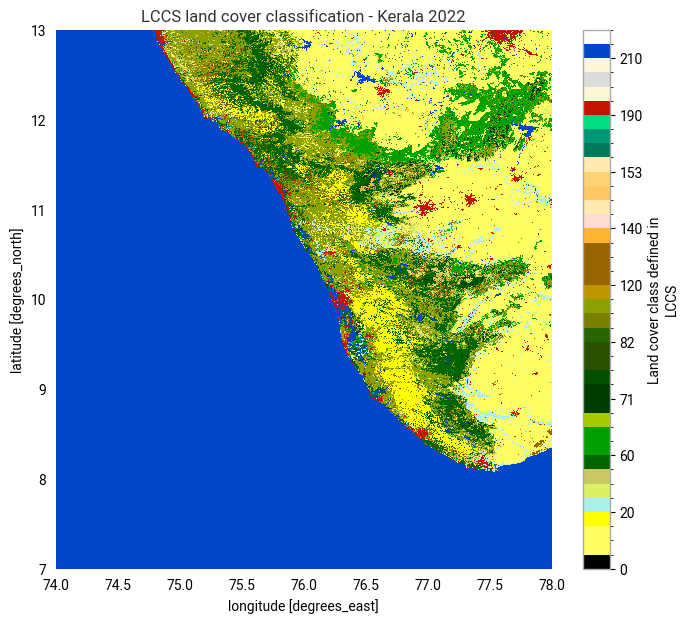
Figure 2: Land Cover map 2022 including the legend for the region Kerala.

# Show the complete dataset
data

<xarray.Dataset> Size: 101GB
Dimensions:              (time: 1, lat: 64800, lon: 129600, bounds: 2)
Coordinates:
  * lat                  (lat) float64 518kB 90.0 90.0 89.99 ... -90.0 -90.0
  * lon                  (lon) float64 1MB -180.0 -180.0 -180.0 ... 180.0 180.0
  * time                 (time) datetime64[ns] 8B 2022-01-01
Dimensions without coordinates: bounds
Data variables:
    lccs_class           (time, lat, lon) uint8 8GB dask.array<chunksize=(1, 2025, 2025), meta=np.ndarray>
    processed_flag       (time, lat, lon) float32 34GB dask.array<chunksize=(1, 2025, 2025), meta=np.ndarray>
    current_pixel_state  (time, lat, lon) float32 34GB dask.array<chunksize=(1, 2025, 2025), meta=np.ndarray>
    observation_count    (time, lat, lon) uint16 17GB dask.array<chunksize=(1, 2025, 2025), meta=np.ndarray>
    change_count         (time, lat, lon) uint8 8GB dask.array<chunksize=(1, 2025, 2025), meta=np.ndarray>
    crs                  int32 4B ...
    lat_bounds           (lat, bounds) float64 1MB dask.array<chunksize=(64800, 2), meta=np.ndarray>
    lon_bounds           (lon, bounds) float64 2MB dask.array<chunksize=(129600, 2), meta=np.ndarray>
    time_bounds          (time, bounds) datetime64[ns] 16B dask.array<chunksize=(1, 2), meta=np.ndarray>
Attributes: (12/38)
    title:                      Land Cover Map of 2022
    summary:                    This dataset characterizes the land cover of ...
    type:                       C3S-LC-L4-LCCS-Map-300m-P1Y
    references:                 https://cds.climate.copernicus.eu/
    institution:                UCLouvain
    contact:                    copernicus-support@ecmwf.int
    ...                         ...
    geospatial_lon_resolution:  0.002778
    id:                         C3S-LC-L4-LCCS-Map-300m-P1Y-2022-v2.1.1
    project:                    EC C3S Land Cover
    source:                     Sentinel-3 OLCI
    geospatial_lon_min:         -180.0
    geospatial_lon_max:         180.0

xarray.Dataset

• Dimensions:
  • time: 1
  • lat: 64800
  • lon: 129600
  • bounds: 2
• Coordinates: (3)
  • lat
    (lat)
    float64
    90.0 90.0 89.99 ... -90.0 -90.0

    units :

    degrees_north

    long_name :

    latitude

    standard_name :

    latitude

    valid_min :

    -90.0

    valid_max :

    90.0

    bounds :

    lat_bounds

    axis :

    Y

    array([ 89.998611,  89.995833,  89.993056, ..., -89.993056, -89.995833,
           -89.998611], shape=(64800,))

  • lon
    (lon)
    float64
    -180.0 -180.0 ... 180.0 180.0

    units :

    degrees_east

    long_name :

    longitude

    standard_name :

    longitude

    valid_min :

    -180.0

    valid_max :

    180.0

    bounds :

    lon_bounds

    axis :

    X

    array([-179.998611, -179.995833, -179.993056, ...,  179.993056,  179.995833,
            179.998611], shape=(129600,))

  • time
    (time)
    datetime64[ns]
    2022-01-01

    standard_name :

    time

    long_name :

    time

    axis :

    T

    bounds :

    time_bounds

    array(['2022-01-01T00:00:00.000000000'], dtype='datetime64[ns]')

• Data variables: (9)
  • lccs_class
    (time, lat, lon)
    uint8
    dask.array<chunksize=(1, 2025, 2025), meta=np.ndarray>

    standard_name :

    land_cover_lccs

    flag_colors :

    #ffff64 #ffff64 #ffff00 #aaf0f0 #dcf064 #c8c864 #006400 #00a000 #00a000 #aac800 #003c00 #003c00 #005000 #285000 #285000 #286400 #788200 #8ca000 #be9600 #966400 #966400 #966400 #ffb432 #ffdcd2 #ffebaf #ffc864 #ffd278 #ffebaf #00785a #009678 #00dc82 #c31400 #fff5d7 #dcdcdc #fff5d7 #0046c8 #ffffff

    long_name :

    Land cover class defined in LCCS

    valid_min :

    1

    valid_max :

    220

    ancillary_variables :

    processed_flag current_pixel_state observation_count change_count

    flag_meanings :

    no_data cropland_rainfed cropland_rainfed_herbaceous_cover cropland_rainfed_tree_or_shrub_cover cropland_irrigated mosaic_cropland mosaic_natural_vegetation tree_broadleaved_evergreen_closed_to_open tree_broadleaved_deciduous_closed_to_open tree_broadleaved_deciduous_closed tree_broadleaved_deciduous_open tree_needleleaved_evergreen_closed_to_open tree_needleleaved_evergreen_closed tree_needleleaved_evergreen_open tree_needleleaved_deciduous_closed_to_open tree_needleleaved_deciduous_closed tree_needleleaved_deciduous_open tree_mixed mosaic_tree_and_shrub mosaic_herbaceous shrubland shrubland_evergreen shrubland_deciduous grassland lichens_and_mosses sparse_vegetation sparse_tree sparse_shrub sparse_herbaceous tree_cover_flooded_fresh_or_brakish_water tree_cover_flooded_saline_water shrub_or_herbaceous_cover_flooded urban bare_areas bare_areas_consolidated bare_areas_unconsolidated water snow_and_ice

    flag_values :

    [ 0 10 11 12 20 30 40 50 60 61 62 70 71 72 80 81 82 90 100 110 120 121 122 130 140 150 151 152 153 160 170 180 190 200 201 202 210 220]

    Array Chunk Bytes 7.82 GiB 3.91 MiB Shape (1, 64800, 129600) (1, 2025, 2025) Dask graph 2048 chunks in 2 graph layers Data type uint8 numpy.ndarray

  • processed_flag
    (time, lat, lon)
    float32
    dask.array<chunksize=(1, 2025, 2025), meta=np.ndarray>

    long_name :

    LC map processed area flag

    standard_name :

    land_cover_lccs status_flag

    valid_min :

    0

    valid_max :

    1

    flag_meanings :

    not_processed processed

    flag_values :

    [0 1]

    Array Chunk Bytes 31.29 GiB 15.64 MiB Shape (1, 64800, 129600) (1, 2025, 2025) Dask graph 2048 chunks in 2 graph layers Data type float32 numpy.ndarray

  • current_pixel_state
    (time, lat, lon)
    float32
    dask.array<chunksize=(1, 2025, 2025), meta=np.ndarray>

    long_name :

    LC pixel type mask

    standard_name :

    land_cover_lccs status_flag

    valid_min :

    0

    valid_max :

    5

    flag_meanings :

    invalid clear_land clear_water clear_snow_ice cloud cloud_shadow

    flag_values :

    [0 1 2 3 4 5]

    Array Chunk Bytes 31.29 GiB 15.64 MiB Shape (1, 64800, 129600) (1, 2025, 2025) Dask graph 2048 chunks in 2 graph layers Data type float32 numpy.ndarray

  • observation_count
    (time, lat, lon)
    uint16
    dask.array<chunksize=(1, 2025, 2025), meta=np.ndarray>

    long_name :

    number of valid observations

    standard_name :

    land_cover_lccs number_of_observations

    valid_min :

    0

    valid_max :

    32767

    Array Chunk Bytes 15.64 GiB 7.82 MiB Shape (1, 64800, 129600) (1, 2025, 2025) Dask graph 2048 chunks in 2 graph layers Data type uint16 numpy.ndarray

  • change_count
    (time, lat, lon)
    uint8
    dask.array<chunksize=(1, 2025, 2025), meta=np.ndarray>

    long_name :

    number of class changes

    valid_min :

    0

    valid_max :

    100

    Array Chunk Bytes 7.82 GiB 3.91 MiB Shape (1, 64800, 129600) (1, 2025, 2025) Dask graph 2048 chunks in 2 graph layers Data type uint8 numpy.ndarray

  • crs
    ()
    int32
    ...

    wkt :

    GEOGCS["WGS 84", DATUM["World Geodetic System 1984", SPHEROID["WGS 84", 6378137.0, 298.257223563, AUTHORITY["EPSG","7030"]], AUTHORITY["EPSG","6326"]], PRIMEM["Greenwich", 0.0, AUTHORITY["EPSG","8901"]], UNIT["degree", 0.017453292519943295], AXIS["Geodetic longitude", EAST], AXIS["Geodetic latitude", NORTH], AUTHORITY["EPSG","4326"]]

    i2m :

    0.002777777777778,0.0,0.0,-0.002777777777778,-180.0,90.0

    [1 values with dtype=int32]

  • lat_bounds
    (lat, bounds)
    float64
    dask.array<chunksize=(64800, 2), meta=np.ndarray>

    Array Chunk Bytes 0.99 MiB 0.99 MiB Shape (64800, 2) (64800, 2) Dask graph 1 chunks in 2 graph layers Data type float64 numpy.ndarray

  • lon_bounds
    (lon, bounds)
    float64
    dask.array<chunksize=(129600, 2), meta=np.ndarray>

    Array Chunk Bytes 1.98 MiB 1.98 MiB Shape (129600, 2) (129600, 2) Dask graph 1 chunks in 2 graph layers Data type float64 numpy.ndarray

  • time_bounds
    (time, bounds)
    datetime64[ns]
    dask.array<chunksize=(1, 2), meta=np.ndarray>

    Array Chunk Bytes 16 B 16 B Shape (1, 2) (1, 2) Dask graph 1 chunks in 2 graph layers Data type datetime64[ns] numpy.ndarray

• Indexes: (3)
  • lat
    PandasIndex

    PandasIndex(Index([ 89.99861111111113,  89.99583333333334,  89.99305555555557,
            89.99027777777778,  89.98750000000001,  89.98472222222222,
            89.98194444444445,  89.97916666666669,  89.97638888888889,
            89.97361111111113,
           ...
           -89.97361111111111, -89.97638888888889, -89.97916666666667,
           -89.98194444444445, -89.98472222222222,           -89.9875,
           -89.99027777777778, -89.99305555555556, -89.99583333333334,
           -89.99861111111112],
          dtype='float64', name='lat', length=64800))

  • lon
    PandasIndex

    PandasIndex(Index([ -179.9986111111111, -179.99583333333334, -179.99305555555554,
           -179.99027777777778,           -179.9875, -179.98472222222222,
           -179.98194444444445, -179.97916666666666,  -179.9763888888889,
            -179.9736111111111,
           ...
             179.9736111111111,   179.9763888888889,  179.97916666666669,
            179.98194444444448,  179.98472222222222,            179.9875,
             179.9902777777778,  179.99305555555554,  179.99583333333334,
            179.99861111111113],
          dtype='float64', name='lon', length=129600))

  • time
    PandasIndex

    PandasIndex(DatetimeIndex(['2022-01-01'], dtype='datetime64[ns]', name='time', freq=None))

• Attributes: (38)

  title :

  Land Cover Map of 2022

  summary :

  This dataset characterizes the land cover of a particular year (see time_coverage). The land cover was derived from the analysis of satellite data time series of the full period.

  type :

  C3S-LC-L4-LCCS-Map-300m-P1Y

  references :

  https://cds.climate.copernicus.eu/

  institution :

  UCLouvain

  contact :

  copernicus-support@ecmwf.int

  comment :

  Conventions :

  CF-1.6

  standard_name_vocabulary :

  NetCDF Climate and Forecast (CF) Standard Names version 21

  keywords :

  land cover classification,satellite,observation

  keywords_vocabulary :

  NASA Global Change Master Directory (GCMD) Science Keywords

  license :

  EC C3S Land cover Data Policy

  naming_authority :

  cdm_data_type :

  grid

  TileSize :

  2025:2025

  tracking_id :

  cbc0983e-a0fd-4277-9023-2e618c0c2067

  product_version :

  2.1.1

  creation_date :

  20240220T123148Z

  creator_name :

  UCLouvain

  creator_url :

  http://www.uclouvain.be/

  creator_email :

  landcover-cci@uclouvain.be

  history :

  lc-sr-1.0, lc-classification-1.0,lc-user-tools-3.14,lc-user-tools-4.5

  time_coverage_start :

  20220101

  time_coverage_end :

  20221231

  time_coverage_duration :

  P1Y

  time_coverage_resolution :

  P1Y

  geospatial_lat_min :

  -90.0

  geospatial_lat_max :

  90.0

  spatial_resolution :

  300m

  geospatial_lat_units :

  degrees_north

  geospatial_lat_resolution :

  0.002778

  geospatial_lon_units :

  degrees_east

  geospatial_lon_resolution :

  0.002778

  id :

  C3S-LC-L4-LCCS-Map-300m-P1Y-2022-v2.1.1

  project :

  EC C3S Land Cover

  source :

  Sentinel-3 OLCI

  geospatial_lon_min :

  -180.0

  geospatial_lon_max :

  180.0

# Show the subset of the dataset
data_lc_2D

<xarray.DataArray 'lccs_class' (time: 1, lat: 2160, lon: 1440)> Size: 3MB
dask.array<getitem, shape=(1, 2160, 1440), dtype=uint8, chunksize=(1, 1530, 1440), chunktype=numpy.ndarray>
Coordinates:
  * lat      (lat) float64 17kB 13.0 13.0 12.99 12.99 ... 7.01 7.007 7.004 7.001
  * lon      (lon) float64 12kB 74.0 74.0 74.01 74.01 ... 77.99 77.99 78.0 78.0
  * time     (time) datetime64[ns] 8B 2022-01-01
Attributes:
    standard_name:        land_cover_lccs
    flag_colors:          #ffff64 #ffff64 #ffff00 #aaf0f0 #dcf064 #c8c864 #00...
    long_name:            Land cover class defined in LCCS
    valid_min:            1
    valid_max:            220
    ancillary_variables:  processed_flag current_pixel_state observation_coun...
    flag_meanings:        no_data cropland_rainfed cropland_rainfed_herbaceou...
    flag_values:          [  0  10  11  12  20  30  40  50  60  61  62  70  7...

xarray.DataArray

'lccs_class'

• time: 1
• lat: 2160
• lon: 1440

• dask.array<chunksize=(1, 630, 1440), meta=np.ndarray>

  Array Chunk Bytes 2.97 MiB 2.10 MiB Shape (1, 2160, 1440) (1, 1530, 1440) Dask graph 2 chunks in 3 graph layers Data type uint8 numpy.ndarray

• Coordinates: (3)
  • lat
    (lat)
    float64
    13.0 13.0 12.99 ... 7.004 7.001

    units :

    degrees_north

    long_name :

    latitude

    standard_name :

    latitude

    valid_min :

    -90.0

    valid_max :

    90.0

    bounds :

    lat_bounds

    axis :

    Y

    array([12.998611, 12.995833, 12.993056, ...,  7.006944,  7.004167,  7.001389],
          shape=(2160,))

  • lon
    (lon)
    float64
    74.0 74.0 74.01 ... 77.99 78.0 78.0

    units :

    degrees_east

    long_name :

    longitude

    standard_name :

    longitude

    valid_min :

    -180.0

    valid_max :

    180.0

    bounds :

    lon_bounds

    axis :

    X

    array([74.001389, 74.004167, 74.006944, ..., 77.993056, 77.995833, 77.998611],
          shape=(1440,))

  • time
    (time)
    datetime64[ns]
    2022-01-01

    standard_name :

    time

    long_name :

    time

    axis :

    T

    bounds :

    time_bounds

    array(['2022-01-01T00:00:00.000000000'], dtype='datetime64[ns]')

• Indexes: (3)
  • lat
    PandasIndex

    PandasIndex(Index([12.998611111111117, 12.995833333333337, 12.993055555555557,
           12.990277777777777, 12.987499999999997, 12.984722222222231,
           12.981944444444451, 12.979166666666671, 12.976388888888891,
           12.973611111111111,
           ...
            7.026388888888889,  7.023611111111109,  7.020833333333343,
            7.018055555555563,  7.015277777777783,  7.012500000000003,
            7.009722222222223,  7.006944444444443,  7.004166666666677,
            7.001388888888897],
          dtype='float64', name='lat', length=2160))

  • lon
    PandasIndex

    PandasIndex(Index([ 74.0013888888889, 74.00416666666666, 74.00694444444446,
           74.00972222222222, 74.01250000000002, 74.01527777777778,
           74.01805555555558, 74.02083333333334, 74.02361111111111,
            74.0263888888889,
           ...
            77.9736111111111, 77.97638888888889, 77.97916666666669,
           77.98194444444448, 77.98472222222222, 77.98750000000001,
            77.9902777777778, 77.99305555555554, 77.99583333333334,
           77.99861111111113],
          dtype='float64', name='lon', length=1440))

  • time
    PandasIndex

    PandasIndex(DatetimeIndex(['2022-01-01'], dtype='datetime64[ns]', name='time', freq=None))

• Attributes: (8)

  standard_name :

  land_cover_lccs

  flag_colors :

  #ffff64 #ffff64 #ffff00 #aaf0f0 #dcf064 #c8c864 #006400 #00a000 #00a000 #aac800 #003c00 #003c00 #005000 #285000 #285000 #286400 #788200 #8ca000 #be9600 #966400 #966400 #966400 #ffb432 #ffdcd2 #ffebaf #ffc864 #ffd278 #ffebaf #00785a #009678 #00dc82 #c31400 #fff5d7 #dcdcdc #fff5d7 #0046c8 #ffffff

  long_name :

  Land cover class defined in LCCS

  valid_min :

  1

  valid_max :

  220

  ancillary_variables :

  processed_flag current_pixel_state observation_count change_count

  flag_meanings :

  no_data cropland_rainfed cropland_rainfed_herbaceous_cover cropland_rainfed_tree_or_shrub_cover cropland_irrigated mosaic_cropland mosaic_natural_vegetation tree_broadleaved_evergreen_closed_to_open tree_broadleaved_deciduous_closed_to_open tree_broadleaved_deciduous_closed tree_broadleaved_deciduous_open tree_needleleaved_evergreen_closed_to_open tree_needleleaved_evergreen_closed tree_needleleaved_evergreen_open tree_needleleaved_deciduous_closed_to_open tree_needleleaved_deciduous_closed tree_needleleaved_deciduous_open tree_mixed mosaic_tree_and_shrub mosaic_herbaceous shrubland shrubland_evergreen shrubland_deciduous grassland lichens_and_mosses sparse_vegetation sparse_tree sparse_shrub sparse_herbaceous tree_cover_flooded_fresh_or_brakish_water tree_cover_flooded_saline_water shrub_or_herbaceous_cover_flooded urban bare_areas bare_areas_consolidated bare_areas_unconsolidated water snow_and_ice

  flag_values :

  [ 0 10 11 12 20 30 40 50 60 61 62 70 71 72 80 81 82 90 100 110 120 121 122 130 140 150 151 152 153 160 170 180 190 200 201 202 210 220]

Write dataset contents to a netCDF file.

data_subset.to_netcdf(
    os.path.join(DATADIR, "lc_2022_kerala.nc")
)

Re-project the data into another projection

Let’s visualise the year 2022 for the Kerala region once again, but in a different projection!

ax = plt.axes(projection=ccrs.Orthographic(80, 10))
ax.set_global()
data_lc_2D[0].plot(ax=ax, transform=ccrs.PlateCarree(),cmap=cmap, norm=norm )
ax.coastlines()
plt.title(title)
plt.show()

Figure 3: Land Cover map 2022 including the legend for the region Kerala - orthographic projection.

Use case I - Explore C3S & CCI Land Cover over time

Application main steps:

• Definition of the time period and download the data

• Define a subset based on the latitude and longitude values

• Show the results and save the image

• Define a point based on the latitude and longitude values

• Show the time series and save the image

# Define a download filename:
download_filename_multiyear = f"{DATADIR}/lc_2016-2022_subset.zip"

# Downloading ba-pixel product over Europe
dataset = "satellite-land-cover"
request = {
    "variable": "all",
    "year": [
        "2016", "2018", "2020",
        "2022"
    ],
    "version": ["v2_1_1"],
    "area": [15, 70, 5, 80],
}

if not os.path.exists(download_filename_multiyear):
    c.retrieve(dataset, request, download_filename_multiyear)
else:
    print(f"File {download_filename_multiyear} already exists. Skipping download.")

lc_data_multiple_years = ek.data.from_source("file", download_filename_multiyear)
lc_data_multiple_years

File ./data_dir//lc_2016-2022_subset.zip already exists. Skipping download.

NetCDFMultiFieldList(NetCDFFieldListReader(C:\Users\Grit\AppData\Local\Temp\tmpkqxyyu5_\file-93f2ae6dd694fdcb5c2665f401f7686e0944aaadb8e64de064c19c612e6e81a2.d\C3S-LC-L4-LCCS-Map-300m-P1Y-2016-v2.1.1.area-subset.15.80.5.70.nc),NetCDFFieldListReader(C:\Users\Grit\AppData\Local\Temp\tmpkqxyyu5_\file-93f2ae6dd694fdcb5c2665f401f7686e0944aaadb8e64de064c19c612e6e81a2.d\C3S-LC-L4-LCCS-Map-300m-P1Y-2018-v2.1.1.area-subset.15.80.5.70.nc),NetCDFFieldListReader(C:\Users\Grit\AppData\Local\Temp\tmpkqxyyu5_\file-93f2ae6dd694fdcb5c2665f401f7686e0944aaadb8e64de064c19c612e6e81a2.d\C3S-LC-L4-LCCS-Map-300m-P1Y-2020-v2.1.1.area-subset.15.80.5.70.nc),NetCDFFieldListReader(C:\Users\Grit\AppData\Local\Temp\tmpkqxyyu5_\file-93f2ae6dd694fdcb5c2665f401f7686e0944aaadb8e64de064c19c612e6e81a2.d\C3S-LC-L4-LCCS-Map-300m-P1Y-2022-v2.1.1.area-subset.15.80.5.70.nc))

# Spatial subset selection 
min_lon = 74
min_lat = 13
max_lon = 78
max_lat = 7

data_multiyear=lc_data_multiple_years.to_xarray()
data_subset = data_multiyear.sel(lat=slice(min_lat,max_lat), lon=slice(min_lon,max_lon))
data_lc_2D=data_subset['lccs_class']

# Set plot title	

time_str_0= str(data_lc_2D.coords['time'].values[0]).split('-')[0]
time_str_1= str(data_lc_2D.coords['time'].values[1]).split('-')[0]
time_str_2= str(data_lc_2D.coords['time'].values[2]).split('-')[0]
time_str_3= str(data_lc_2D.coords['time'].values[3]).split('-')[0]
title = 'LCCS land cover classification - Kerala'

# Create the figure
fig, ((ax0, ax1), (ax2, ax3)) = plt.subplots(2, 2, constrained_layout = True)
fig.suptitle(title)
# fig.tight_layout()
# fig.subplots_adjust(top=0.88)
data_lc_2D[0].plot(cmap=cmap, norm=norm, ax=ax0)
ax0.set_title(time_str_0)
data_lc_2D[1].plot(cmap=cmap, norm=norm, ax=ax1)
ax1.set_title(time_str_1)
data_lc_2D[2].plot(cmap=cmap, norm=norm, ax=ax2)
ax2.set_title(time_str_2)
data_lc_2D[3].plot(cmap=cmap, norm=norm, ax=ax3)
ax3.set_title(time_str_3)

# Show figure
plt.show()

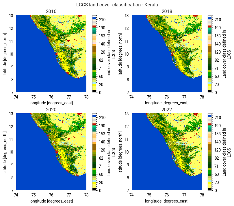
Figure 4: Land Cover map 2016, 2018, 2020 & 2022 including the legend for the region Kerala.

# Show the dataset
data

<xarray.Dataset> Size: 101GB
Dimensions:              (time: 1, lat: 64800, lon: 129600, bounds: 2)
Coordinates:
  * lat                  (lat) float64 518kB 90.0 90.0 89.99 ... -90.0 -90.0
  * lon                  (lon) float64 1MB -180.0 -180.0 -180.0 ... 180.0 180.0
  * time                 (time) datetime64[ns] 8B 2022-01-01
Dimensions without coordinates: bounds
Data variables:
    lccs_class           (time, lat, lon) uint8 8GB dask.array<chunksize=(1, 2025, 2025), meta=np.ndarray>
    processed_flag       (time, lat, lon) float32 34GB dask.array<chunksize=(1, 2025, 2025), meta=np.ndarray>
    current_pixel_state  (time, lat, lon) float32 34GB dask.array<chunksize=(1, 2025, 2025), meta=np.ndarray>
    observation_count    (time, lat, lon) uint16 17GB dask.array<chunksize=(1, 2025, 2025), meta=np.ndarray>
    change_count         (time, lat, lon) uint8 8GB dask.array<chunksize=(1, 2025, 2025), meta=np.ndarray>
    crs                  int32 4B ...
    lat_bounds           (lat, bounds) float64 1MB dask.array<chunksize=(64800, 2), meta=np.ndarray>
    lon_bounds           (lon, bounds) float64 2MB dask.array<chunksize=(129600, 2), meta=np.ndarray>
    time_bounds          (time, bounds) datetime64[ns] 16B dask.array<chunksize=(1, 2), meta=np.ndarray>
Attributes: (12/38)
    title:                      Land Cover Map of 2022
    summary:                    This dataset characterizes the land cover of ...
    type:                       C3S-LC-L4-LCCS-Map-300m-P1Y
    references:                 https://cds.climate.copernicus.eu/
    institution:                UCLouvain
    contact:                    copernicus-support@ecmwf.int
    ...                         ...
    geospatial_lon_resolution:  0.002778
    id:                         C3S-LC-L4-LCCS-Map-300m-P1Y-2022-v2.1.1
    project:                    EC C3S Land Cover
    source:                     Sentinel-3 OLCI
    geospatial_lon_min:         -180.0
    geospatial_lon_max:         180.0

xarray.Dataset

• Dimensions:
  • time: 1
  • lat: 64800
  • lon: 129600
  • bounds: 2
• Coordinates: (3)
  • lat
    (lat)
    float64
    90.0 90.0 89.99 ... -90.0 -90.0

    units :

    degrees_north

    long_name :

    latitude

    standard_name :

    latitude

    valid_min :

    -90.0

    valid_max :

    90.0

    bounds :

    lat_bounds

    axis :

    Y

    array([ 89.998611,  89.995833,  89.993056, ..., -89.993056, -89.995833,
           -89.998611], shape=(64800,))

  • lon
    (lon)
    float64
    -180.0 -180.0 ... 180.0 180.0

    units :

    degrees_east

    long_name :

    longitude

    standard_name :

    longitude

    valid_min :

    -180.0

    valid_max :

    180.0

    bounds :

    lon_bounds

    axis :

    X

    array([-179.998611, -179.995833, -179.993056, ...,  179.993056,  179.995833,
            179.998611], shape=(129600,))

  • time
    (time)
    datetime64[ns]
    2022-01-01

    standard_name :

    time

    long_name :

    time

    axis :

    T

    bounds :

    time_bounds

    array(['2022-01-01T00:00:00.000000000'], dtype='datetime64[ns]')

• Data variables: (9)
  • lccs_class
    (time, lat, lon)
    uint8
    dask.array<chunksize=(1, 2025, 2025), meta=np.ndarray>

    standard_name :

    land_cover_lccs

    flag_colors :

    #ffff64 #ffff64 #ffff00 #aaf0f0 #dcf064 #c8c864 #006400 #00a000 #00a000 #aac800 #003c00 #003c00 #005000 #285000 #285000 #286400 #788200 #8ca000 #be9600 #966400 #966400 #966400 #ffb432 #ffdcd2 #ffebaf #ffc864 #ffd278 #ffebaf #00785a #009678 #00dc82 #c31400 #fff5d7 #dcdcdc #fff5d7 #0046c8 #ffffff

    long_name :

    Land cover class defined in LCCS

    valid_min :

    1

    valid_max :

    220

    ancillary_variables :

    processed_flag current_pixel_state observation_count change_count

    flag_meanings :

    no_data cropland_rainfed cropland_rainfed_herbaceous_cover cropland_rainfed_tree_or_shrub_cover cropland_irrigated mosaic_cropland mosaic_natural_vegetation tree_broadleaved_evergreen_closed_to_open tree_broadleaved_deciduous_closed_to_open tree_broadleaved_deciduous_closed tree_broadleaved_deciduous_open tree_needleleaved_evergreen_closed_to_open tree_needleleaved_evergreen_closed tree_needleleaved_evergreen_open tree_needleleaved_deciduous_closed_to_open tree_needleleaved_deciduous_closed tree_needleleaved_deciduous_open tree_mixed mosaic_tree_and_shrub mosaic_herbaceous shrubland shrubland_evergreen shrubland_deciduous grassland lichens_and_mosses sparse_vegetation sparse_tree sparse_shrub sparse_herbaceous tree_cover_flooded_fresh_or_brakish_water tree_cover_flooded_saline_water shrub_or_herbaceous_cover_flooded urban bare_areas bare_areas_consolidated bare_areas_unconsolidated water snow_and_ice

    flag_values :

    [ 0 10 11 12 20 30 40 50 60 61 62 70 71 72 80 81 82 90 100 110 120 121 122 130 140 150 151 152 153 160 170 180 190 200 201 202 210 220]

    Array Chunk Bytes 7.82 GiB 3.91 MiB Shape (1, 64800, 129600) (1, 2025, 2025) Dask graph 2048 chunks in 2 graph layers Data type uint8 numpy.ndarray

  • processed_flag
    (time, lat, lon)
    float32
    dask.array<chunksize=(1, 2025, 2025), meta=np.ndarray>

    long_name :

    LC map processed area flag

    standard_name :

    land_cover_lccs status_flag

    valid_min :

    0

    valid_max :

    1

    flag_meanings :

    not_processed processed

    flag_values :

    [0 1]

    Array Chunk Bytes 31.29 GiB 15.64 MiB Shape (1, 64800, 129600) (1, 2025, 2025) Dask graph 2048 chunks in 2 graph layers Data type float32 numpy.ndarray

  • current_pixel_state
    (time, lat, lon)
    float32
    dask.array<chunksize=(1, 2025, 2025), meta=np.ndarray>

    long_name :

    LC pixel type mask

    standard_name :

    land_cover_lccs status_flag

    valid_min :

    0

    valid_max :

    5

    flag_meanings :

    invalid clear_land clear_water clear_snow_ice cloud cloud_shadow

    flag_values :

    [0 1 2 3 4 5]

    Array Chunk Bytes 31.29 GiB 15.64 MiB Shape (1, 64800, 129600) (1, 2025, 2025) Dask graph 2048 chunks in 2 graph layers Data type float32 numpy.ndarray

  • observation_count
    (time, lat, lon)
    uint16
    dask.array<chunksize=(1, 2025, 2025), meta=np.ndarray>

    long_name :

    number of valid observations

    standard_name :

    land_cover_lccs number_of_observations

    valid_min :

    0

    valid_max :

    32767

    Array Chunk Bytes 15.64 GiB 7.82 MiB Shape (1, 64800, 129600) (1, 2025, 2025) Dask graph 2048 chunks in 2 graph layers Data type uint16 numpy.ndarray

  • change_count
    (time, lat, lon)
    uint8
    dask.array<chunksize=(1, 2025, 2025), meta=np.ndarray>

    long_name :

    number of class changes

    valid_min :

    0

    valid_max :

    100

    Array Chunk Bytes 7.82 GiB 3.91 MiB Shape (1, 64800, 129600) (1, 2025, 2025) Dask graph 2048 chunks in 2 graph layers Data type uint8 numpy.ndarray

  • crs
    ()
    int32
    ...

    wkt :

    GEOGCS["WGS 84", DATUM["World Geodetic System 1984", SPHEROID["WGS 84", 6378137.0, 298.257223563, AUTHORITY["EPSG","7030"]], AUTHORITY["EPSG","6326"]], PRIMEM["Greenwich", 0.0, AUTHORITY["EPSG","8901"]], UNIT["degree", 0.017453292519943295], AXIS["Geodetic longitude", EAST], AXIS["Geodetic latitude", NORTH], AUTHORITY["EPSG","4326"]]

    i2m :

    0.002777777777778,0.0,0.0,-0.002777777777778,-180.0,90.0

    [1 values with dtype=int32]

  • lat_bounds
    (lat, bounds)
    float64
    dask.array<chunksize=(64800, 2), meta=np.ndarray>

    Array Chunk Bytes 0.99 MiB 0.99 MiB Shape (64800, 2) (64800, 2) Dask graph 1 chunks in 2 graph layers Data type float64 numpy.ndarray

  • lon_bounds
    (lon, bounds)
    float64
    dask.array<chunksize=(129600, 2), meta=np.ndarray>

    Array Chunk Bytes 1.98 MiB 1.98 MiB Shape (129600, 2) (129600, 2) Dask graph 1 chunks in 2 graph layers Data type float64 numpy.ndarray

  • time_bounds
    (time, bounds)
    datetime64[ns]
    dask.array<chunksize=(1, 2), meta=np.ndarray>

    Array Chunk Bytes 16 B 16 B Shape (1, 2) (1, 2) Dask graph 1 chunks in 2 graph layers Data type datetime64[ns] numpy.ndarray

• Indexes: (3)
  • lat
    PandasIndex

    PandasIndex(Index([ 89.99861111111113,  89.99583333333334,  89.99305555555557,
            89.99027777777778,  89.98750000000001,  89.98472222222222,
            89.98194444444445,  89.97916666666669,  89.97638888888889,
            89.97361111111113,
           ...
           -89.97361111111111, -89.97638888888889, -89.97916666666667,
           -89.98194444444445, -89.98472222222222,           -89.9875,
           -89.99027777777778, -89.99305555555556, -89.99583333333334,
           -89.99861111111112],
          dtype='float64', name='lat', length=64800))

  • lon
    PandasIndex

    PandasIndex(Index([ -179.9986111111111, -179.99583333333334, -179.99305555555554,
           -179.99027777777778,           -179.9875, -179.98472222222222,
           -179.98194444444445, -179.97916666666666,  -179.9763888888889,
            -179.9736111111111,
           ...
             179.9736111111111,   179.9763888888889,  179.97916666666669,
            179.98194444444448,  179.98472222222222,            179.9875,
             179.9902777777778,  179.99305555555554,  179.99583333333334,
            179.99861111111113],
          dtype='float64', name='lon', length=129600))

  • time
    PandasIndex

    PandasIndex(DatetimeIndex(['2022-01-01'], dtype='datetime64[ns]', name='time', freq=None))

• Attributes: (38)

  title :

  Land Cover Map of 2022

  summary :

  This dataset characterizes the land cover of a particular year (see time_coverage). The land cover was derived from the analysis of satellite data time series of the full period.

  type :

  C3S-LC-L4-LCCS-Map-300m-P1Y

  references :

  https://cds.climate.copernicus.eu/

  institution :

  UCLouvain

  contact :

  copernicus-support@ecmwf.int

  comment :

  Conventions :

  CF-1.6

  standard_name_vocabulary :

  NetCDF Climate and Forecast (CF) Standard Names version 21

  keywords :

  land cover classification,satellite,observation

  keywords_vocabulary :

  NASA Global Change Master Directory (GCMD) Science Keywords

  license :

  EC C3S Land cover Data Policy

  naming_authority :

  cdm_data_type :

  grid

  TileSize :

  2025:2025

  tracking_id :

  cbc0983e-a0fd-4277-9023-2e618c0c2067

  product_version :

  2.1.1

  creation_date :

  20240220T123148Z

  creator_name :

  UCLouvain

  creator_url :

  http://www.uclouvain.be/

  creator_email :

  landcover-cci@uclouvain.be

  history :

  lc-sr-1.0, lc-classification-1.0,lc-user-tools-3.14,lc-user-tools-4.5

  time_coverage_start :

  20220101

  time_coverage_end :

  20221231

  time_coverage_duration :

  P1Y

  time_coverage_resolution :

  P1Y

  geospatial_lat_min :

  -90.0

  geospatial_lat_max :

  90.0

  spatial_resolution :

  300m

  geospatial_lat_units :

  degrees_north

  geospatial_lat_resolution :

  0.002778

  geospatial_lon_units :

  degrees_east

  geospatial_lon_resolution :

  0.002778

  id :

  C3S-LC-L4-LCCS-Map-300m-P1Y-2022-v2.1.1

  project :

  EC C3S Land Cover

  source :

  Sentinel-3 OLCI

  geospatial_lon_min :

  -180.0

  geospatial_lon_max :

  180.0

# Show the subset of the dataset
data_lc_2D

<xarray.DataArray 'lccs_class' (time: 4, lat: 2160, lon: 1440)> Size: 12MB
dask.array<getitem, shape=(4, 2160, 1440), dtype=uint8, chunksize=(1, 2160, 1440), chunktype=numpy.ndarray>
Coordinates:
  * lat      (lat) float64 17kB 13.0 13.0 12.99 12.99 ... 7.01 7.007 7.004 7.001
  * lon      (lon) float64 12kB 74.0 74.0 74.01 74.01 ... 77.99 77.99 78.0 78.0
  * time     (time) datetime64[ns] 32B 2016-01-01 2018-01-01 ... 2022-01-01
Attributes:
    standard_name:        land_cover_lccs
    flag_colors:          #ffff64 #ffff64 #ffff00 #aaf0f0 #dcf064 #c8c864 #00...
    long_name:            Land cover class defined in LCCS
    valid_min:            1
    valid_max:            220
    ancillary_variables:  processed_flag current_pixel_state observation_coun...
    flag_meanings:        no_data cropland_rainfed cropland_rainfed_herbaceou...
    flag_values:          [  0  10  11  12  20  30  40  50  60  61  62  70  7...

xarray.DataArray

'lccs_class'

• time: 4
• lat: 2160
• lon: 1440

• dask.array<chunksize=(1, 2160, 1440), meta=np.ndarray>

  Array Chunk Bytes 11.87 MiB 2.97 MiB Shape (4, 2160, 1440) (1, 2160, 1440) Dask graph 4 chunks in 10 graph layers Data type uint8 numpy.ndarray

• Coordinates: (3)
  • lat
    (lat)
    float64
    13.0 13.0 12.99 ... 7.004 7.001

    units :

    degrees_north

    long_name :

    latitude

    standard_name :

    latitude

    valid_min :

    -90.0

    valid_max :

    90.0

    bounds :

    lat_bounds

    axis :

    Y

    array([12.998611, 12.995833, 12.993056, ...,  7.006944,  7.004167,  7.001389],
          shape=(2160,))

  • lon
    (lon)
    float64
    74.0 74.0 74.01 ... 77.99 78.0 78.0

    units :

    degrees_east

    long_name :

    longitude

    standard_name :

    longitude

    valid_min :

    -180.0

    valid_max :

    180.0

    bounds :

    lon_bounds

    axis :

    X

    array([74.001389, 74.004167, 74.006944, ..., 77.993056, 77.995833, 77.998611],
          shape=(1440,))

  • time
    (time)
    datetime64[ns]
    2016-01-01 ... 2022-01-01

    standard_name :

    time

    long_name :

    time

    axis :

    T

    bounds :

    time_bounds

    array(['2016-01-01T00:00:00.000000000', '2018-01-01T00:00:00.000000000',
           '2020-01-01T00:00:00.000000000', '2022-01-01T00:00:00.000000000'],
          dtype='datetime64[ns]')

• Indexes: (3)
  • lat
    PandasIndex

    PandasIndex(Index([12.998611111111117, 12.995833333333337, 12.993055555555557,
           12.990277777777777, 12.987499999999997, 12.984722222222231,
           12.981944444444451, 12.979166666666671, 12.976388888888891,
           12.973611111111111,
           ...
            7.026388888888889,  7.023611111111109,  7.020833333333343,
            7.018055555555563,  7.015277777777783,  7.012500000000003,
            7.009722222222223,  7.006944444444443,  7.004166666666677,
            7.001388888888897],
          dtype='float64', name='lat', length=2160))

  • lon
    PandasIndex

    PandasIndex(Index([ 74.0013888888889, 74.00416666666666, 74.00694444444446,
           74.00972222222222, 74.01250000000002, 74.01527777777778,
           74.01805555555558, 74.02083333333334, 74.02361111111111,
            74.0263888888889,
           ...
            77.9736111111111, 77.97638888888889, 77.97916666666669,
           77.98194444444448, 77.98472222222222, 77.98750000000001,
            77.9902777777778, 77.99305555555554, 77.99583333333334,
           77.99861111111113],
          dtype='float64', name='lon', length=1440))

  • time
    PandasIndex

    PandasIndex(DatetimeIndex(['2016-01-01', '2018-01-01', '2020-01-01', '2022-01-01'], dtype='datetime64[ns]', name='time', freq=None))

• Attributes: (8)

  standard_name :

  land_cover_lccs

  flag_colors :

  #ffff64 #ffff64 #ffff00 #aaf0f0 #dcf064 #c8c864 #006400 #00a000 #00a000 #aac800 #003c00 #003c00 #005000 #285000 #285000 #286400 #788200 #8ca000 #be9600 #966400 #966400 #966400 #ffb432 #ffdcd2 #ffebaf #ffc864 #ffd278 #ffebaf #00785a #009678 #00dc82 #c31400 #fff5d7 #dcdcdc #fff5d7 #0046c8 #ffffff

  long_name :

  Land cover class defined in LCCS

  valid_min :

  1

  valid_max :

  220

  ancillary_variables :

  processed_flag current_pixel_state observation_count change_count

  flag_meanings :

  no_data cropland_rainfed cropland_rainfed_herbaceous_cover cropland_rainfed_tree_or_shrub_cover cropland_irrigated mosaic_cropland mosaic_natural_vegetation tree_broadleaved_evergreen_closed_to_open tree_broadleaved_deciduous_closed_to_open tree_broadleaved_deciduous_closed tree_broadleaved_deciduous_open tree_needleleaved_evergreen_closed_to_open tree_needleleaved_evergreen_closed tree_needleleaved_evergreen_open tree_needleleaved_deciduous_closed_to_open tree_needleleaved_deciduous_closed tree_needleleaved_deciduous_open tree_mixed mosaic_tree_and_shrub mosaic_herbaceous shrubland shrubland_evergreen shrubland_deciduous grassland lichens_and_mosses sparse_vegetation sparse_tree sparse_shrub sparse_herbaceous tree_cover_flooded_fresh_or_brakish_water tree_cover_flooded_saline_water shrub_or_herbaceous_cover_flooded urban bare_areas bare_areas_consolidated bare_areas_unconsolidated water snow_and_ice

  flag_values :

  [ 0 10 11 12 20 30 40 50 60 61 62 70 71 72 80 81 82 90 100 110 120 121 122 130 140 150 151 152 153 160 170 180 190 200 201 202 210 220]

# Point selection
lon = 76.179167
lat = 10.401389

data_subset = data_multiyear.sel(lat=lat, lon=lon, method='nearest')
data_lc_timeseries=data_subset['lccs_class']

time=np.ones(4, dtype=int)
values=np.ones(4, dtype=int)
for i in range(4):
    time[i]= int(str(data_lc_timeseries.coords['time'].values[i]).split('-')[0])
    values[i]= data_lc_timeseries[i]

title = 'Temporal Variation of LCCS land cover class for Kerala at a chosen location: '

# Create the figure
fig, ax = plt.subplots()
ax.plot(time, values,  marker="D", linestyle='None', color ='red')
ax.set_xlim(2015, 2023)
ax.set_ylim(0, 255)
ax.set_title(title + 'point lat:' + str(lat) + '° lon:' + str(lon) + '°')
ax.set_ylabel("Land cover class defined in LCCS")
ax.set_xlabel("year")
# Show figure
plt.show()

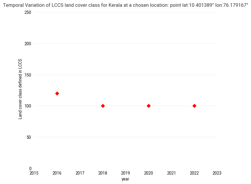
Figure 5: LCCS Land Cover class on a selected location in Kerala for the years 2016, 2018, 2020 & 2022. The figure plots the LCC number (y-axis) over time (x-axis). The time series of the C3S and CCI land cover maps (CLC) at this location shows a change in the LCCS land cover class.

Use case II - Examine regional statistics of C3S & CCI Land Cover information

Application main steps:

• Select a region based on the shape file

• Show the results and save the image

• Calculate the regional statistics and show/save the results

Here we are using the LC 2022 map data and country borders provided by Nomenclature of territorial units for statistics (NUTS).

First we will download and open the NUTS with earthkit.data, the output from the cell below shows the first 10 rows of the geopandas representation of the NUTS shapes.

# Access the GISCO NUTS 2024 dataset with earthkit
nuts_2024 = ek.data.from_source(
    "url", "https://gisco-services.ec.europa.eu/distribution/v2/nuts/geojson/NUTS_RG_60M_2024_4326_LEVL_0.geojson"
)
nuts_gpd = nuts_2024.to_geopandas()
# Set the index to the NUTS_ID column
nuts_gpd.set_index("NUTS_ID", inplace=True)
nuts_gpd[:10]

	LEVL_CODE	CNTR_CODE	NAME_LATN	NUTS_NAME	MOUNT_TYPE	URBN_TYPE	COAST_TYPE	geometry
NUTS_ID
EL	0	EL	Elláda	Ελλάδα	NaN	None	None	MULTIPOLYGON (((28.13811 36.32213, 27.83164 35...
ES	0	ES	España	España	NaN	None	None	MULTIPOLYGON (((4.31657 39.87646, 4.20006 39.8...
FI	0	FI	Suomi/Finland	Suomi/Finland	NaN	None	None	MULTIPOLYGON (((28.92956 69.05191, 28.49493 68...
FR	0	FR	France	France	NaN	None	None	MULTIPOLYGON (((55.86434 -21.24704, 55.49022 -...
HR	0	HR	Hrvatska	Hrvatska	NaN	None	None	MULTIPOLYGON (((16.5968 46.4759, 16.85475 46.3...
HU	0	HU	Magyarország	Magyarország	NaN	None	None	POLYGON ((21.38824 48.5496, 22.12108 48.37831,...
IE	0	IE	Éire/Ireland	Éire/Ireland	NaN	None	None	POLYGON ((-8.04432 54.36347, -7.42482 54.1433,...
IS	0	IS	Ísland	Ísland	NaN	None	None	MULTIPOLYGON (((-15.04445 66.15393, -13.86672 ...
AL	0	AL	Shqipëria	Shqipëria	NaN	None	None	POLYGON ((20.0763 42.55582, 20.36436 42.3066, ...
AT	0	AT	Österreich	Österreich	NaN	None	None	POLYGON ((16.94028 48.61725, 16.94978 48.53579...

We can now use earthkit.transforms to mask the data, we choose to only mask the "lccs_class" variable and set the mask_dim to the "NUTS_ID" column of the geopandas above. The output in the cell below shows our masked data array, there is a new dimension, NUTS_ID which corresponds to each of the countries in the NUTS dataset.

country = "Finland"
nuts_id = "FI"
nuts_gpd_subset = nuts_gpd.loc[[nuts_id]]
min_lon, min_lat, max_lon, max_lat = nuts_gpd_subset.bounds.values[0] 

global_lccs_data = lc_data.to_xarray()["lccs_class"]
# Subset to bounds of our gpd
subset_lccs_data = global_lccs_data.sel(
    lat=slice(max_lat, min_lat), lon=slice(min_lon, max_lon)
)
# subset_lccs_data
# Mask the data
data_lccs_masked = ek.transforms.aggregate.spatial.mask(
    subset_lccs_data, nuts_gpd_subset, mask_dim="NUTS_ID", all_touched=True
)
data_lccs_masked

<xarray.DataArray 'lccs_class' (NUTS_ID: 1, time: 1, lat: 3672, lon: 4298)> Size: 63MB
dask.array<broadcast_to, shape=(1, 1, 3672, 4298), dtype=float32, chunksize=(1, 1, 2025, 2025), chunktype=numpy.ndarray>
Coordinates:
  * lat      (lat) float64 29kB 70.05 70.05 70.05 70.04 ... 59.86 59.86 59.85
  * lon      (lon) float64 34kB 19.52 19.53 19.53 19.53 ... 31.45 31.46 31.46
  * time     (time) datetime64[ns] 8B 2022-01-01
  * NUTS_ID  (NUTS_ID) object 8B 'FI'
Attributes:
    standard_name:        land_cover_lccs
    flag_colors:          #ffff64 #ffff64 #ffff00 #aaf0f0 #dcf064 #c8c864 #00...
    long_name:            Land cover class defined in LCCS
    valid_min:            1
    valid_max:            220
    ancillary_variables:  processed_flag current_pixel_state observation_coun...
    flag_meanings:        no_data cropland_rainfed cropland_rainfed_herbaceou...
    flag_values:          [  0  10  11  12  20  30  40  50  60  61  62  70  7...

xarray.DataArray

'lccs_class'

• NUTS_ID: 1
• time: 1
• lat: 3672
• lon: 4298

• dask.array<chunksize=(1, 1, 919, 1072), meta=np.ndarray>

  Array Chunk Bytes 60.20 MiB 15.64 MiB Shape (1, 1, 3672, 4298) (1, 1, 2025, 2025) Dask graph 9 chunks in 8 graph layers Data type float32 numpy.ndarray

• Coordinates: (4)
  • lat
    (lat)
    float64
    70.05 70.05 70.05 ... 59.86 59.85

    units :

    degrees_north

    long_name :

    latitude

    standard_name :

    latitude

    valid_min :

    -90.0

    valid_max :

    90.0

    bounds :

    lat_bounds

    axis :

    Y

    array([70.051389, 70.048611, 70.045833, ..., 59.859722, 59.856944, 59.854167],
          shape=(3672,))

  • lon
    (lon)
    float64
    19.52 19.53 19.53 ... 31.46 31.46

    units :

    degrees_east

    long_name :

    longitude

    standard_name :

    longitude

    valid_min :

    -180.0

    valid_max :

    180.0

    bounds :

    lon_bounds

    axis :

    X

    array([19.523611, 19.526389, 19.529167, ..., 31.454167, 31.456944, 31.459722],
          shape=(4298,))

  • time
    (time)
    datetime64[ns]
    2022-01-01

    standard_name :

    time

    long_name :

    time

    axis :

    T

    bounds :

    time_bounds

    array(['2022-01-01T00:00:00.000000000'], dtype='datetime64[ns]')

  • NUTS_ID
    (NUTS_ID)
    object
    'FI'

    array(['FI'], dtype=object)

• Indexes: (4)
  • lat
    PandasIndex

    PandasIndex(Index([ 70.05138888888891,  70.04861111111111,  70.04583333333335,
            70.04305555555555,  70.04027777777779,            70.0375,
            70.03472222222223,  70.03194444444446,  70.02916666666667,
             70.0263888888889,
           ...
            59.87916666666666,   59.8763888888889,   59.8736111111111,
            59.87083333333334,  59.86805555555557,  59.86527777777778,
            59.86250000000001,  59.85972222222222,  59.85694444444445,
           59.854166666666686],
          dtype='float64', name='lat', length=3672))

  • lon
    PandasIndex

    PandasIndex(Index([ 19.52361111111111, 19.526388888888903,  19.52916666666667,
           19.531944444444463,  19.53472222222223, 19.537499999999994,
            19.54027777777779, 19.543055555555554,  19.54583333333335,
           19.548611111111114,
           ...
           31.434722222222234,            31.4375, 31.440277777777794,
            31.44305555555556, 31.445833333333354,  31.44861111111112,
           31.451388888888886,  31.45416666666668, 31.456944444444446,
            31.45972222222224],
          dtype='float64', name='lon', length=4298))

  • time
    PandasIndex

    PandasIndex(DatetimeIndex(['2022-01-01'], dtype='datetime64[ns]', name='time', freq=None))

  • NUTS_ID
    PandasIndex

    PandasIndex(Index(['FI'], dtype='object', name='NUTS_ID'))

• Attributes: (8)

  standard_name :

  land_cover_lccs

  flag_colors :

  #ffff64 #ffff64 #ffff00 #aaf0f0 #dcf064 #c8c864 #006400 #00a000 #00a000 #aac800 #003c00 #003c00 #005000 #285000 #285000 #286400 #788200 #8ca000 #be9600 #966400 #966400 #966400 #ffb432 #ffdcd2 #ffebaf #ffc864 #ffd278 #ffebaf #00785a #009678 #00dc82 #c31400 #fff5d7 #dcdcdc #fff5d7 #0046c8 #ffffff

  long_name :

  Land cover class defined in LCCS

  valid_min :

  1

  valid_max :

  220

  ancillary_variables :

  processed_flag current_pixel_state observation_count change_count

  flag_meanings :

  no_data cropland_rainfed cropland_rainfed_herbaceous_cover cropland_rainfed_tree_or_shrub_cover cropland_irrigated mosaic_cropland mosaic_natural_vegetation tree_broadleaved_evergreen_closed_to_open tree_broadleaved_deciduous_closed_to_open tree_broadleaved_deciduous_closed tree_broadleaved_deciduous_open tree_needleleaved_evergreen_closed_to_open tree_needleleaved_evergreen_closed tree_needleleaved_evergreen_open tree_needleleaved_deciduous_closed_to_open tree_needleleaved_deciduous_closed tree_needleleaved_deciduous_open tree_mixed mosaic_tree_and_shrub mosaic_herbaceous shrubland shrubland_evergreen shrubland_deciduous grassland lichens_and_mosses sparse_vegetation sparse_tree sparse_shrub sparse_herbaceous tree_cover_flooded_fresh_or_brakish_water tree_cover_flooded_saline_water shrub_or_herbaceous_cover_flooded urban bare_areas bare_areas_consolidated bare_areas_unconsolidated water snow_and_ice

  flag_values :

  [ 0 10 11 12 20 30 40 50 60 61 62 70 71 72 80 81 82 90 100 110 120 121 122 130 140 150 151 152 153 160 170 180 190 200 201 202 210 220]

# Show and save the image with applied mask  
# Set plot title
country = 'Finland'
nuts_id = 'FI'
time_str= str(data_lccs_masked.coords['time'].values[0]).split('-')[0]
title = f'LCCS land cover classification map  - {country} {time_str}'

data_lccs_region = data_lccs_masked.isel(time=0)
# Create the figure
data_lccs_region.plot(cmap=cmap, norm=norm)
plt.title(title)
# Show figure
plt.show()

Figure 6: Land Cover map 2022 including the legend for the Finland.

# area of the polygon
area_polygon = nuts_gpd_subset.area.head()
area_polygon

C:\Users\Grit\AppData\Local\Temp\ipykernel_26588\2147410973.py:2: UserWarning: Geometry is in a geographic CRS. Results from 'area' are likely incorrect. Use 'GeoSeries.to_crs()' to re-project geometries to a projected CRS before this operation.

  area_polygon = nuts_gpd_subset.area.head()

NUTS_ID
FI    63.850359
dtype: float64

# Create & plot a histogram
classes = np.array([0, 10, 11, 12, 20, 30, 40, 50, 60, 61, 62, 70, 71, 72, 80,
        81, 82, 90, 100, 110, 120, 121, 122, 130, 140, 150, 151,
        152, 153, 160, 170, 180, 190, 200, 201, 202, 210, 220, 230])
min_edge = classes - 0.2
max_edge= classes + 0.2
range = (-5, 235)
data_lccs_region_1D=data_lccs_masked.stack(z=('lat', 'lon')).reset_index('z')
data_lccs_region_1D_series = data_lccs_region_1D.to_series()
data_lccs_region_1D_series_len_without_nan = data_lccs_region_1D_series.size-np.isnan(data_lccs_region_1D_series).sum()
data_lccs_region_1D_series.dropna(inplace=True)

fig, ax = plt.subplots(nrows=1, ncols=1, figsize=(10, 5))
xr.plot.hist(
    data_lccs_region_1D, range=range, bins=classes,
    ax=ax, histtype='bar', color='blue'
)
ax.set_title("Land Cover Classification Histogram")
ax.set_ylabel("number of occurrences - frequency")
ax.set_ylim([0, 4.5E6])
plt.show()

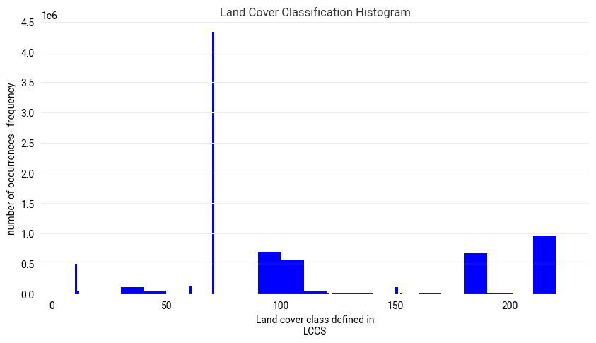
Figure 7: Histogram of Land Cover map 2022 over the classes for Finland showing the number of occurrences - frequency (y-axis) for each LCCS LC class (x-axis).

# N is the count in each bin, bins is the lower-limit of the bin
N, bins = np.histogram(data_lccs_region_1D_series, bins=classes)
N_norm, bins_norm = np.histogram(data_lccs_region_1D_series, bins=classes, density=True)

# Calulate area per pixel
area_per_pixel= area_polygon/len(data_lccs_region_1D_series)
area_per_class_a = N_norm * float(area_polygon[0])
area_per_class_b = N * float(area_per_pixel[0])

class_labels = ["  0 - No Data",
" 10 - Cropland, rainfed",
" 11 - Cropland, rainfed, herbaceous cover",
" 12 - Cropland, rainfed, tree, or shrub cover",
" 20 - Cropland, irrigated or post-flooding",
" 30 - Mosaic cropland (>50%) / natural vegetation (tree, shrub, herbaceous cover) (<50%)",
" 40 - Mosaic natural vegetation (tree, shrub, herbaceous cover) (>50%) / cropland (<50%)",
" 50 - Tree cover, broadleaved, evergreen, closed to open (>15%)",
" 60 - Tree cover, broadleaved, deciduous, closed to open (>15%)",
" 61 - Tree cover, broadleaved, deciduous, closed (>40%)",
" 62 - Tree cover, broadleaved, deciduous, open (15-40%)",
" 70 - Tree cover, needleleaved, evergreen, closed to open (>15%)",
" 71 - Tree cover, needleleaved, evergreen, closed (>40%)",
" 72 - Tree cover, needleleaved, evergreen, open (15-40%)",
" 80 - Tree cover, needleleaved, deciduous, closed to open (>15%)",
" 81 - Tree cover, needleleaved, deciduous, closed (>40%)",
" 82 - Tree cover, needleleaved, deciduous, open (15-40%)",
" 90 - Tree cover, mixed leaf type (broadleaved and needleleaved)",
"100 - Mosaic tree and shrub (>50%) / herbaceous cover (<50%)",
"110 - Mosaic herbaceous cover (>50%) / tree and shrub (<50%)",
"120 - Shrubland",
"121 - Evergreen shrubland",
"122 - Deciduous shrubland",
"130 - Grassland",
"140 - Lichens and mosses",
"150 - Sparse vegetation (tree, shrub, herbaceous cover) (<15%)",
"151 - Sparse tree (<15%)",
"152 - Sparse shrub (<15%)",
"153 - Sparse herbaceous cover (<15%)",
"160 - Tree cover, flooded, fresh, or brackish water",
"170 - Tree cover, flooded, saline water",
"180 - Shrub or herbaceous cover, flooded, fresh/saline/brackish water",
"190 - Urban areas",
"200 - Bare areas",
"201 - Consolidated bare areas",
"202 - Unconsolidated bare areas",
"210 - Water bodies",
"220 - Permanent snow and ice"]

colors = ((0, 0, 0),                 # 0
         (1, 1, 0.392156),           # 10
         (1, 1, 0.392156),           # 11
         (1, 1, 0),                  # 12
         (0.666666, 0.941176, 0.941176),    # 20
         (0.862745, 0.941176, 0.392156),    # 30
         (0.784313, 0.784313, 0.392156),    # 40
         (0, 0.392156, 0),           # 50
         (0, 0.62745, 0),            # 60
         (0, 0.62745, 0),            # 61
         (0.666666, 0.784313, 0),    # 62
         (0, 0.235294, 0),           # 70
         (0, 0.235294, 0),           # 71
         (0, 0.313725, 0),           # 72
         (0.156862, 0.313725, 0),    # 80
         (0.156862, 0.313725, 0),    # 81
         (0.156862, 0.392156, 0),    # 82
         (0.470588, 0.509803, 0),    # 90
         (0.549019, 0.62745, 0),     # 100
         (0.745098, 0.588235, 0),    # 110
         (0.588235, 0.392156, 0),    # 120
         (0.588235, 0.392156, 0),    # 121
         (0.588235, 0.392156, 0),    # 122
         (1, 0.705882, 0.196078),    # 130
         (1, 0.862745, 0.823529),    # 140
         (1, 0.921568, 0.686274),    # 150
         (1, 0.784313, 0.392156),    # 151
         (1, 0.823529, 0.470588),    # 152
         (1, 0.921568, 0.686274),    # 153
         (0, 0.470588, 0.352941),    # 160
         (0, 0.588235, 0.470588),    # 170
         (0, 0.862745, 0.509803),    # 180
         (0.764705, 0.078431, 0),    # 190
         (1, 0.960784, 0.843137),    # 200
         (0.862745, 0.862745, 0.862745),    # 201
         (1, 0.960784, 0.843137),    # 202
         (0, 0.274509, 0.784313),   # 210
         (1, 1, 1)    # 220
         )

df_area = pd.DataFrame(classes[0:len(classes)-1], columns=['LCCS'])
df_area["class_labels"] = class_labels
df_area["numbers"] = N
df_area["numbers_norm"] = N_norm
df_area["percent"] = N_norm * 100.
df_area["percent_2_nd_version"] = N/np.sum(N) * 100.
df_area["area_per_class"]=area_per_class_a
df_area["area_per_class_2nd_version"]=area_per_class_b

display(df_area)

C:\Users\Grit\AppData\Local\Temp\ipykernel_26588\436065005.py:7: FutureWarning: Series.__getitem__ treating keys as positions is deprecated. In a future version, integer keys will always be treated as labels (consistent with DataFrame behavior). To access a value by position, use `ser.iloc[pos]`
  area_per_class_a = N_norm * float(area_polygon[0])
C:\Users\Grit\AppData\Local\Temp\ipykernel_26588\436065005.py:8: FutureWarning: Series.__getitem__ treating keys as positions is deprecated. In a future version, integer keys will always be treated as labels (consistent with DataFrame behavior). To access a value by position, use `ser.iloc[pos]`
  area_per_class_b = N * float(area_per_pixel[0])

	LCCS	class_labels	numbers	numbers_norm	percent	percent_2_nd_version	area_per_class	area_per_class_2nd_version
0	0	0 - No Data	0	0.000000	0.000000	0.000000	0.000000	0.000000
1	10	10 - Cropland, rainfed	492537	0.059437	5.943738	5.943738	3.795098	3.795098
2	11	11 - Cropland, rainfed, herbaceous cover	56794	0.006854	0.685367	0.685367	0.437609	0.437609
3	12	12 - Cropland, rainfed, tree, or shrub cover	0	0.000000	0.000000	0.000000	0.000000	0.000000
4	20	20 - Cropland, irrigated or post-flooding	0	0.000000	0.000000	0.000000	0.000000	0.000000
5	30	30 - Mosaic cropland (>50%) / natural vegetat...	105869	0.001278	0.127758	1.277584	0.081574	0.815742
6	40	40 - Mosaic natural vegetation (tree, shrub, ...	56001	0.000676	0.067580	0.675797	0.043150	0.431499
7	50	50 - Tree cover, broadleaved, evergreen, clos...	0	0.000000	0.000000	0.000000	0.000000	0.000000
8	60	60 - Tree cover, broadleaved, deciduous, clos...	136647	0.016490	1.649001	1.649001	1.052893	1.052893
9	61	61 - Tree cover, broadleaved, deciduous, clos...	0	0.000000	0.000000	0.000000	0.000000	0.000000
10	62	62 - Tree cover, broadleaved, deciduous, open...	0	0.000000	0.000000	0.000000	0.000000	0.000000
11	70	70 - Tree cover, needleleaved, evergreen, clo...	4335691	0.523214	52.321371	52.321371	33.407383	33.407383
12	71	71 - Tree cover, needleleaved, evergreen, clo...	0	0.000000	0.000000	0.000000	0.000000	0.000000
13	72	72 - Tree cover, needleleaved, evergreen, ope...	0	0.000000	0.000000	0.000000	0.000000	0.000000
14	80	80 - Tree cover, needleleaved, deciduous, clo...	147	0.000018	0.001774	0.001774	0.001133	0.001133
15	81	81 - Tree cover, needleleaved, deciduous, clo...	0	0.000000	0.000000	0.000000	0.000000	0.000000
16	82	82 - Tree cover, needleleaved, deciduous, ope...	0	0.000000	0.000000	0.000000	0.000000	0.000000
17	90	90 - Tree cover, mixed leaf type (broadleaved...	685195	0.008269	0.826866	8.268657	0.527957	5.279567
18	100	100 - Mosaic tree and shrub (>50%) / herbaceou...	552176	0.006663	0.666344	6.663437	0.425463	4.254629
19	110	110 - Mosaic herbaceous cover (>50%) / tree an...	56559	0.000683	0.068253	0.682531	0.043580	0.435799
20	120	120 - Shrubland	8944	0.001079	0.107933	0.107933	0.068915	0.068915
21	121	121 - Evergreen shrubland	0	0.000000	0.000000	0.000000	0.000000	0.000000
22	122	122 - Deciduous shrubland	5218	0.000079	0.007871	0.062969	0.005026	0.040206
23	130	130 - Grassland	1269	0.000015	0.001531	0.015314	0.000978	0.009778
24	140	140 - Lichens and mosses	0	0.000000	0.000000	0.000000	0.000000	0.000000
25	150	150 - Sparse vegetation (tree, shrub, herbaceo...	116048	0.014004	1.400420	1.400420	0.894174	0.894174
26	151	151 - Sparse tree (<15%)	0	0.000000	0.000000	0.000000	0.000000	0.000000
27	152	152 - Sparse shrub (<15%)	9386	0.001133	0.113266	0.113266	0.072321	0.072321
28	153	153 - Sparse herbaceous cover (<15%)	0	0.000000	0.000000	0.000000	0.000000	0.000000
29	160	160 - Tree cover, flooded, fresh, or brackish ...	641	0.000008	0.000774	0.007735	0.000494	0.004939
30	170	170 - Tree cover, flooded, saline water	0	0.000000	0.000000	0.000000	0.000000	0.000000
31	180	180 - Shrub or herbaceous cover, flooded, fres...	674972	0.008145	0.814529	8.145290	0.520080	5.200797
32	190	190 - Urban areas	19300	0.000233	0.023290	0.232905	0.014871	0.148710
33	200	200 - Bare areas	10134	0.001223	0.122293	0.122293	0.078085	0.078085
34	201	201 - Consolidated bare areas	48	0.000006	0.000579	0.000579	0.000370	0.000370
35	202	202 - Unconsolidated bare areas	0	0.000000	0.000000	0.000000	0.000000	0.000000
36	210	210 - Water bodies	963078	0.011622	1.162204	11.622037	0.742071	7.420712
37	220	220 - Permanent snow and ice	0	0.000000	0.000000	0.000000	0.000000	0.000000

Table 1: Regional statistics of Land Cover map over the LCCS land cover classes for Finland 2022.

# Save statistics
file_name_statistics= os.path.join(DATADIR, f"lc_2022_{country}.csv")
df_area.to_csv(file_name_statistics, sep=';', index=False)

# Set plot title
time_str= str(data_lccs_masked.coords['time'].values[0]).split('-')[0]
title = f'Bar chart - LCCS landcover classification -  {country.title()} {time_str}'

# Create the figures
fig, ax = plt.subplots(1, 1, tight_layout=True)

ax.bar(np.char.mod('%d', df_area['LCCS'].values), df_area["numbers_norm"].values,  color=colors)
# Now we format the y-axis to display percentage
# ax.yaxis.set_major_formatter(PercentFormatter(xmax=1))
ax.set_title(title)
ax.tick_params(axis='x', labelrotation=90)
# ax.legend(title='LCCS', loc='upper center', ncol=2)
ax.set_ylim([0, 1])
ax.set_xlabel("Land cover class defined in LCCS")
ax.set_ylabel("proportion")

plt.show()

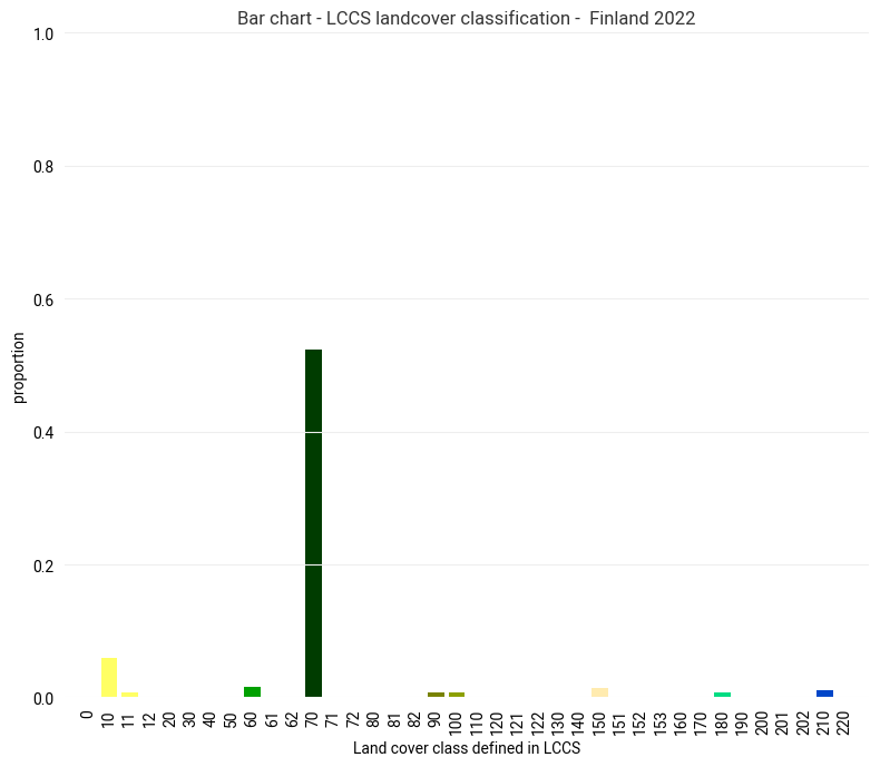
Figure 8: Normalized histogram of Land Cover map 2022 over the LCCS land cover classes for Finland, showing the proportion of the country’s land surface (y-axis) under each identified LCCS LC class (x-axis).

Conclusion

You can use land cover data available through the Copernicus Climate Change Service (C3S) to explore global and regional changes over time. This tutorial demonstrated how C3S and CCI Land Cover products available through the C3S can be explored using a Jupyter Notebook, and the information available. By producing spatial statistics of the LCCS classes, we produced information on Finland’s Land Cover. We have downloaded, visualised, subset, and analysed the data, to produce meaningful and informative visuals and tables. In addition, we derived and visualised an additional aspect - land cover change - from the data.