
Analysis of September 2020 European heatwave using ERA5 climate reanalysis data from C3S#
This notebook can be run on free online platforms, such as Binder, Kaggle and Colab, or they can be accessed from GitHub. The links to run this notebook in these environments are provided here, but please note they are not supported by ECMWF.
![]()

![]()
Learning objectives 🎯#
In September 2020, a record-breaking heatwave occured in large parts of western Europe, (see a description here). The city of Lille in northern France for example experienced its hottest day in September 2020 since records began in 1945. In this tutorial we will analyse this event with data from the Climate Data Store (CDS) of the Copernicus Climate Change Service (C3S).
In this tutorial, we will:
View daily maximum 2m temperature for September 2020
Compare maximum temperatures with climatology
Prepare your environment#
(Install and) Import libraries#
We will be working with data in NetCDF format. To best handle this data we will use libraries for working with multidimensional arrays, in particular Xarray. We will also need libraries for plotting and viewing data, in this case we will use Matplotlib and Cartopy.
# Earthkit
import earthkit as ek
import earthkit.plots

# Library for interacting with the operating system
import os

# Libraries for working with multidimensional arrays
import numpy as np
import xarray as xr

# Libraries for plotting and visualising data
import matplotlib.path as mpath
import matplotlib.pyplot as plt
import cartopy.crs as ccrs
from cartopy.mpl.gridliner import LONGITUDE_FORMATTER, LATITUDE_FORMATTER
import cartopy.feature as cfeature

# Disable warnings for data download via API
import urllib3
urllib3.disable_warnings()
Explore data#
To search for data, visit the CDS website: https://cds.climate.copernicus.eu. To facilitate your search you can use keywords, or apply various filters. The data we are going to use in this exercise is the ERA5 reanalysis data on single levels from 1979 to present.
Search for the data#
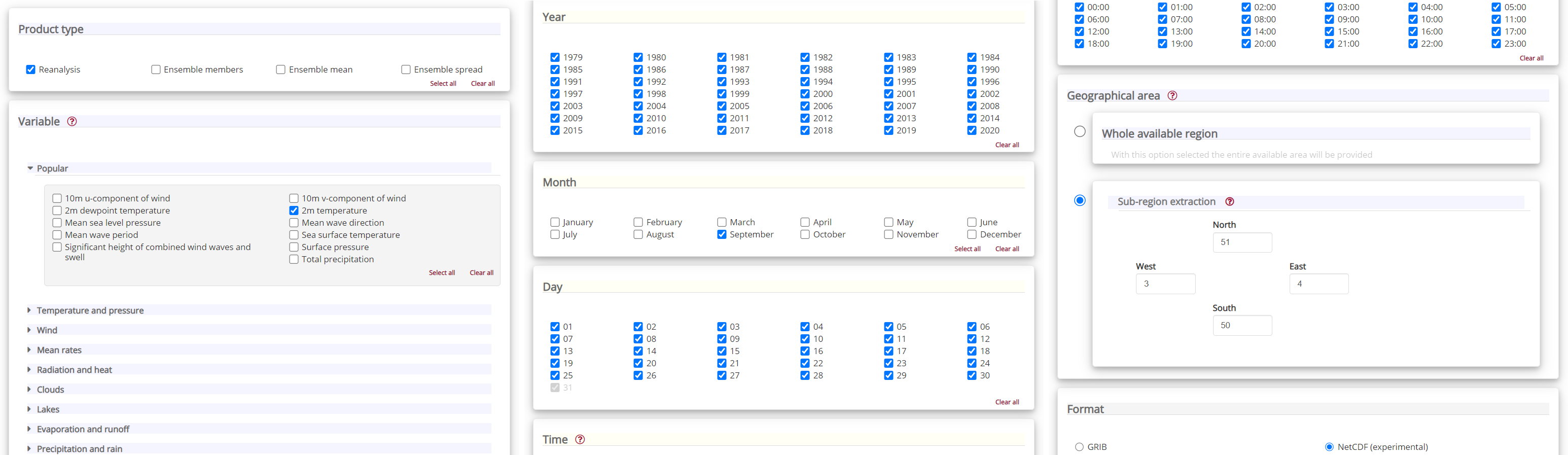
Having selected the correct dataset, we now need to specify what product type, variables, temporal and geographic coverage we are interested in. These can all be selected in the “Download data” tab. In this tab a form appears in which we will select the following parameters to download. We will choose a subset area of 1x1 degrees, corresponding to a region of around 111km North/South and 72km East/West in Belgium and Northern France, around the city of Lille:
Parameters of data to download
Product type:
ReanalysisVariable:
2m temperatureYear:
allMonth:
SeptemberDay:
allTime:
allGeographical area:
North: 51,East: 4,South: 50,West: 3Format:
NetCDF
At the end of the download forms, select “Show API request”. This will reveal a block of code, which you can simply copy and paste into a cell of your Jupyter Notebook (see cell below). Having copied the API request into the cell below, running this will retrieve and download the data you requested into your local directory.
Warning
Please remember to accept the terms and conditions of the dataset, at the bottom of the CDS download form!
Download the data#
With the API request copied into the cell below, running this cell will retrieve and download the data you requested into your local directory.
source = 'cds'
dataset = 'reanalysis-era5-single-levels'
request = {
        'product_type': 'reanalysis',
        'data_format': 'netcdf',
        'variable': '2m_temperature',
        'year': [
            '1991', '1992', '1993',
            '1994', '1995', '1996',
            '1997', '1998', '1999',
            '2000', '2001', '2002',
            '2003', '2004', '2005',
            '2006', '2007', '2008',
            '2009', '2010', '2011',
            '2012', '2013', '2014',
            '2015', '2016', '2017',
            '2018', '2019', '2020',
        ],
        'month': '09',
        'day': [
            '01', '02', '03',
            '04', '05', '06',
            '07', '08', '09',
            '10', '11', '12',
            '13', '14', '15',
            '16', '17', '18',
            '19', '20', '21',
            '22', '23', '24',
            '25', '26', '27',
            '28', '29', '30',
        ],
        'time': [
            '00:00', '01:00', '02:00',
            '03:00', '04:00', '05:00',
            '06:00', '07:00', '08:00',
            '09:00', '10:00', '11:00',
            '12:00', '13:00', '14:00',
            '15:00', '16:00', '17:00',
            '18:00', '19:00', '20:00',
            '21:00', '22:00', '23:00',
        ],
        'area': [
            51, 3, 50,
            4,
        ],
    }
data = earthkit.data.from_source(source,dataset,request)
2025-07-15 11:17:31,468 INFO [2024-09-26T00:00:00] Watch our [Forum](https://forum.ecmwf.int/) for Announcements, news and other discussed topics.
2025-07-15 11:17:31,906 INFO [2024-09-26T00:00:00] Watch our [Forum](https://forum.ecmwf.int/) for Announcements, news and other discussed topics.
---------------------------------------------------------------------------
HTTPError                                 Traceback (most recent call last)
Cell In[13], line 47
      2 dataset = 'reanalysis-era5-single-levels'
      3 request = {
      4         'product_type': 'reanalysis',
      5         'data_format': 'netcdf',
   (...)
     45         ],
     46     }
---> 47 data = earthkit.data.from_source(source,dataset,request)

File /Library/Frameworks/Python.framework/Versions/3.12/lib/python3.12/site-packages/earthkit/data/sources/__init__.py:158, in from_source(name, lazily, *args, **kwargs)
    155     return from_source_lazily(name, *args, **kwargs)
    157 prev = None
--> 158 src = get_source(name, *args, **kwargs)
    159 while src is not prev:
    160     prev = src

File /Library/Frameworks/Python.framework/Versions/3.12/lib/python3.12/site-packages/earthkit/data/sources/__init__.py:139, in SourceMaker.__call__(self, name, *args, **kwargs)
    136     klass = find_plugin(os.path.dirname(__file__), name, loader)
    137     self.SOURCES[name] = klass
--> 139 source = klass(*args, **kwargs)
    141 if getattr(source, "name", None) is None:
    142     source.name = name

File /Library/Frameworks/Python.framework/Versions/3.12/lib/python3.12/site-packages/earthkit/data/core/__init__.py:22, in MetaBase.__call__(cls, *args, **kwargs)
     20 obj = cls.__new__(cls, *args, **kwargs)
     21 args, kwargs = cls.patch(obj, *args, **kwargs)
---> 22 obj.__init__(*args, **kwargs)
     23 return obj

File /Library/Frameworks/Python.framework/Versions/3.12/lib/python3.12/site-packages/earthkit/data/sources/cds.py:126, in CdsRetriever.__init__(self, dataset, prompt, *args, **kwargs)
    123 nthreads = min(self.config("number-of-download-threads"), len(self.requests))
    125 if nthreads < 2:
--> 126     self.path = [self._retrieve(dataset, r) for r in self.requests]
    127 else:
    128     with SoftThreadPool(nthreads=nthreads) as pool:

File /Library/Frameworks/Python.framework/Versions/3.12/lib/python3.12/site-packages/earthkit/data/sources/cds.py:140, in CdsRetriever._retrieve(self, dataset, request)
    137     self.source_filename = cds_result.location.split("/")[-1]
    138     cds_result.download(target=target)
--> 140 return_object = self.cache_file(
    141     retrieve,
    142     (dataset, request),
    143     extension=EXTENSIONS.get(request.get("format"), ".cache"),
    144 )
    145 return return_object

File /Library/Frameworks/Python.framework/Versions/3.12/lib/python3.12/site-packages/earthkit/data/sources/__init__.py:68, in Source.cache_file(self, create, args, **kwargs)
     65 if owner is None:
     66     owner = re.sub(r"(?!^)([A-Z]+)", r"-\1", self.__class__.__name__).lower()
---> 68 return cache_file(owner, create, args, **kwargs)

File /Library/Frameworks/Python.framework/Versions/3.12/lib/python3.12/site-packages/earthkit/data/core/caching.py:1056, in cache_file(owner, create, args, hash_extra, extension, force, replace)
   1054 with FileLock(lock):
   1055     if not os.path.exists(path):  # Check again, another thread/process may have created the file
-> 1056         owner_data = create(path + ".tmp", args)
   1057         os.rename(path + ".tmp", path)
   1058 try:

File /Library/Frameworks/Python.framework/Versions/3.12/lib/python3.12/site-packages/earthkit/data/sources/cds.py:136, in CdsRetriever._retrieve.<locals>.retrieve(target, args)
    135 def retrieve(target, args):
--> 136     cds_result = self.client().retrieve(args[0], args[1])
    137     self.source_filename = cds_result.location.split("/")[-1]
    138     cds_result.download(target=target)

File /Library/Frameworks/Python.framework/Versions/3.12/lib/python3.12/site-packages/datapi/legacy_api_client.py:169, in LegacyApiClient.retrieve(self, name, request, target)
    167 submitted: Remote | Results
    168 if self.wait_until_complete:
--> 169     submitted = self.client.submit_and_wait_on_results(
    170         collection_id=name,
    171         **request,
    172     )
    173 else:
    174     submitted = self.client.submit(
    175         collection_id=name,
    176         **request,
    177     )

File /Library/Frameworks/Python.framework/Versions/3.12/lib/python3.12/site-packages/datapi/api_client.py:458, in ApiClient.submit_and_wait_on_results(self, collection_id, **request)
    442 def submit_and_wait_on_results(
    443     self, collection_id: str, **request: Any
    444 ) -> datapi.Results:
    445     """Submit a request and wait for the results to be ready.
    446
    447     Parameters
   (...)
    456     datapi.Results
    457     """
--> 458     return self._retrieve_api.submit(collection_id, **request).make_results()

File /Library/Frameworks/Python.framework/Versions/3.12/lib/python3.12/site-packages/datapi/processing.py:727, in Processing.submit(self, collection_id, **request)
    726 def submit(self, collection_id: str, **request: Any) -> Remote:
--> 727     return self.get_process(collection_id).submit(**request)

File /Library/Frameworks/Python.framework/Versions/3.12/lib/python3.12/site-packages/datapi/processing.py:319, in Process.submit(self, **request)
    307 def submit(self, **request: Any) -> datapi.Remote:
    308     """Submit a request.
    309
    310     Parameters
   (...)
    317     datapi.Remote
    318     """
--> 319     job = Job.from_request(
    320         "post",
    321         f"{self.url}/execution",
    322         json={"inputs": request},
    323         **self._request_kwargs,
    324     )
    325     return job.make_remote()

File /Library/Frameworks/Python.framework/Versions/3.12/lib/python3.12/site-packages/datapi/processing.py:177, in ApiResponse.from_request(cls, method, url, headers, session, retry_options, request_options, download_options, sleep_max, cleanup, log_callback, log_messages, **kwargs)
    172 response = robust_request(
    173     method, url, headers=headers, **request_options, **kwargs
    174 )
    175 log(logging.DEBUG, f"REPLY {response.text}", callback=log_callback)
--> 177 cads_raise_for_status(response)
    179 self = cls(
    180     response,
    181     headers=headers,
   (...)
    188     log_callback=log_callback,
    189 )
    190 if log_messages:

File /Library/Frameworks/Python.framework/Versions/3.12/lib/python3.12/site-packages/datapi/processing.py:100, in cads_raise_for_status(response)
     93     else:
     94         message = "\n".join(
     95             [
     96                 f"{response.status_code} Client Error: {response.reason} for url: {response.url}",
     97                 error_json_to_message(error_json),
     98             ]
     99         )
--> 100         raise requests.HTTPError(message, response=response)
    101 response.raise_for_status()

HTTPError: 403 Client Error: Forbidden for url: https://cds.climate.copernicus.eu/api/retrieve/v1/processes/reanalysis-era5-single-levels/execution
cost limits exceeded
Your request is too large, please reduce your selection.
Inspect data#
We have requested the data in NetCDF format. This is a commonly used format for array-oriented scientific data. To read and process this data we will make use of the Xarray library. Xarray is an open source project and Python package that makes working with labelled multi-dimensional arrays simple and efficient. We will read the data from our NetCDF file into an xarray.Dataset.
# Create Xarray Dataset
ds = data.to_xarray()
Now we can query our newly created Xarray dataset …
ds
<xarray.Dataset> Size: 6MB
Dimensions:    (longitude: 5, latitude: 5, time: 30240)
Coordinates:
  * longitude  (longitude) float32 20B 3.0 3.25 3.5 3.75 4.0
  * latitude   (latitude) float32 20B 51.0 50.75 50.5 50.25 50.0
  * time       (time) datetime64[ns] 242kB 1979-09-01 ... 2020-09-30T23:00:00
Data variables:
    t2m        (time, latitude, longitude) float64 6MB ...
Attributes:
    Conventions:  CF-1.6
history: 2025-07-09 02:16:23 GMT by grib_to_netcdf-2.41.0: grib_to_n...We see that the dataset has one variable called “t2m”, which stands for “2 metre temperature”, and three coordinates of longitude, latitude and time.
Select the icons to the right of the table above to expand the attributes of the coordinates and data variables. What are the units of the temperature data?
While an Xarray dataset may contain multiple variables, an Xarray data array holds a single variable (which may still be multi-dimensional) and its coordinates. To make the processing of the t2m data easier, we convert in into an Xarray data array:
da = ds['t2m']
Let’s convert the units of the 2m temperature data from Kelvin to degrees Celsius. The formula for this is simple: degrees Celsius = Kelvin - 273.15
t2m_C = da - 273.15
View daily maximum 2m temperature for September 2020#
As a next step, let us visualize the daily maximum 2m air temperature for September 2020. From the graph, we should be able to identify which day in September was hottest in the area around Lille.
First we average over the subset area:
Note
The size covered by each data point varies as a function of latitude. We need to take this into account when averaging. One way to do this is to use the cosine of the latitude as a proxy for the varying sizes.
weights = np.cos(np.deg2rad(t2m_C.latitude))
weights.name = "weights"
t2m_C_weighted = t2m_C.weighted(weights)
Lille_t2m = t2m_C_weighted.mean(["longitude", "latitude"])
Now we select only the data for 2020:
Lille_2020 = Lille_t2m.sel(time='2020')
We can now calculate the max daily 2m temperature for each day in September 2020:
Lille_2020_max = Lille_2020.groupby('time.day').max('time')
Let’s plot the results in a chart:
fig, ax = plt.subplots(1, 1, figsize = (12, 6))

ax.plot(Lille_2020_max.day, Lille_2020_max)
ax.set_title('Max daily t2m for Sep 2020 in Lille region')
ax.set_ylabel('° C')
ax.set_xlabel('day')
ax.grid(linestyle='--')
for i,j in zip(Lille_2020_max.day, np.around(Lille_2020_max.values, 0).astype(int)):
    ax.annotate(str(j),xy=(i,j))
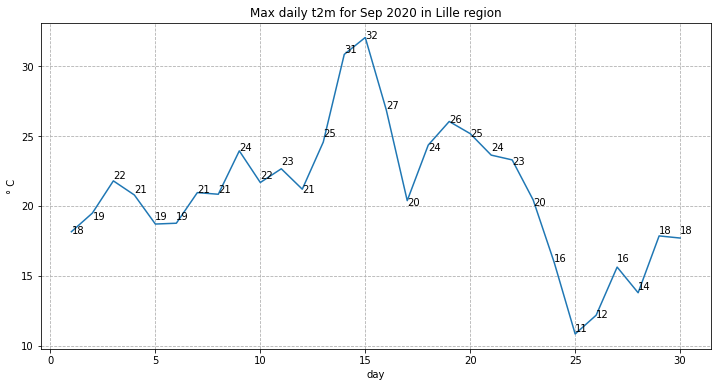
print('The maximum temperature in September 2020 in this area was',
      np.around(Lille_2020_max.max().values, 1), 'degrees Celsius.')
The maximum temperature in September 2020 in this area was 32.1 degrees Celsius.
Which day in September had the highest maximum temperature?
Is this typical for Northern France? How does this compare with the long term average? We will seek to answer these questions in the next section.
Compare maximum temperatures with climatology#
We will now seek to discover just how high the temperature for Lille in mid September 2020 was when compared with typical values exptected in this region at this time of year. To do that we will calculate the climatology of maximum daily 2m temperature for each day in September for the period of 1979 to 2019, and compare these with our values for 2020.
First we select all data prior to 2020:
Lille_past = Lille_t2m.loc['1979':'2019']
Now we calculate the climatology for this data, i.e. the average values for each of the days in September for a period of several decades (from 1979 to 2019).
To do this, we first have to extract the maximum daily value for each day in the time series:
Lille_max = Lille_past.resample(time='D').max().dropna('time')
We will then calculate various quantiles of the maximum daily 2m temperatures for the 40 year time series for each day in September:
Lille_max_max = Lille_max.groupby('time.day').max()
Lille_max_min = Lille_max.groupby('time.day').min()
Lille_max_mid = Lille_max.groupby('time.day').quantile(0.5)
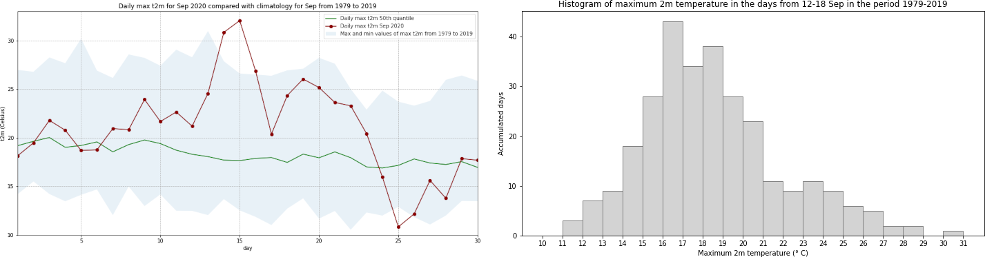
Let’s plot this data. We will plot the, maximum, minimum and 50th quantile of the maximum daily temperature to have an idea of the expected range in this part of France in September, and compare this range with the values for 2020:
fig = plt.figure(figsize=(16,8))
ax = plt.subplot()

ax.plot(Lille_2020_max.day, Lille_max_mid, color='green', label='Daily max t2m 50th quantile')
ax.plot(Lille_2020_max.day, Lille_2020_max, 'bo-', color='darkred', label='Daily max t2m Sep 2020')
ax.fill_between(Lille_2020_max.day, Lille_max_max, Lille_max_min, alpha=0.1,
                label='Max and min values of max t2m from 1979 to 2019')

ax.set_xlim(1,30)
ax.set_ylim(10,33)
ax.set_title('Daily max t2m for Sep 2020 compared with climatology for Sep from 1979 to 2019')
ax.set_ylabel('t2m (Celsius)')
ax.set_xlabel('day')
handles, labels = ax.get_legend_handles_labels()
ax.legend(handles, labels)
ax.grid(linestyle='--')

fig.savefig(f'{DATADIR}Max_t2m_clim_Sep_Lille.png')
C:\Users\cxcs\AppData\Local\Temp/ipykernel_5360/21074062.py:5: UserWarning: color is redundantly defined by the 'color' keyword argument and the fmt string "bo-" (-> color='b'). The keyword argument will take precedence.
  ax.plot(Lille_2020_max.day, Lille_2020_max, 'bo-', color='darkred', label='Daily max t2m Sep 2020')
Interestingly, we see from this plot that while the temperatures from 14 to 16 Sep 2020 were the highest in the ERA5 dataset, on 25 September 2020, the lowest of the maximum temperatures was recorded for this dataset.
We will now look more closely at the probability distribution of maximum temperatures for 15 September in this time period. To do this, we will first select only the max daily temperature for 15 September, for each year in the time series:
Lille_max = Lille_max.dropna('time', how='all')
Lille_15 = Lille_max[14::30]
We will then plot the histogram of this:
Lille_15.plot.hist()
(array([ 2.,  3., 11.,  6.,  7.,  5.,  1.,  2.,  3.,  1.]),
 array([12.54313564, 13.95039225, 15.35764885, 16.76490545, 18.17216206,
        19.57941866, 20.98667526, 22.39393187, 23.80118847, 25.20844507,
        26.61570168]),
 <BarContainer object of 10 artists>)
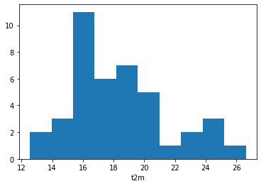
Look at the range of maximum temperatures for 15 September in the period from 1979 to 2019. Has the temperature in this period ever exceeded that of 15 September 2020?
The histogram shows the distribution of maximum temperature of one day in each year of the time series, which corresponds to 41 samples. In order to increase the number of samples, let’s plot the histogram of maximum temperatures on 15 September, plus or minus three days. This would increase our number of samples by a factor of seven.
To do this, we first need to produce an index that takes the maximum 2m air temperature values from 12 to 18 September (15 September +/- three days) from every year in the time series. The first step is to initiate three numpy arrays:
years: with the number of years [0:40]days_in_sep: index values of day range [11:17]index: empty numpy array with 287 (41 years * 7) entries
years = np.arange(41)
days_in_sep = np.arange(11,18)
index = np.zeros(287)
In a next step, we then loop through each entry of the years array and fill the empty index array year by year with the correct indices of the day ranges for each year. The resulting array contains the index values of interest.
for i in years:
    index[i*7:(i*7)+7] = days_in_sep + (i*30)
index = index.astype(int)
We then apply this index to filter the array of max daily temperature from 1979 to 2019. The resulting object is an array of values representing the maximum 2m air temperature in Lille between 12 and 18 September for each year from 1979 to 2019:
Lille_7days = Lille_max.values[index]
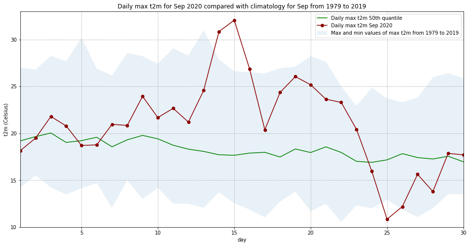
Now we can plot the histogram of maximum daily temperatures in the days 12-18 September from 1979-2019:
fig, ax = plt.subplots(1, 1, figsize = (12, 6))

ax.hist(Lille_7days, bins = np.arange(10,32,1), color='lightgrey', ec='grey')
ax.set_title('Histogram of maximum 2m temperature in the days from 12-18 Sep in the period 1979-2019')
ax.set_xticks(np.arange(10,32,1))
ax.set_ylabel('Accumulated days')
ax.set_xlabel('Maximum 2m temperature (° C)')

fig.savefig(f'{DATADIR}Hist_max_t2m_mid-Sep_1979-2019.png')
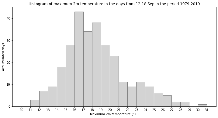
In the histogram above, you see that even if we take an increased sample covering a wider temporal range, the maximum daily temperature still never reached that of 15 September 2020. To increase the sample even further, you could include data from a longer time period. The C3S reanalysis dataset now extends back to 1940 and is accessible here ERA5 hourly data on single levels from 1940 to present.