
Calculation of global climatology of Earth radiation budget from EUMETSAT’s CM SAF CLARA-A3 dataset#
This notebook can be run on free online platforms, such as Binder, Kaggle and Colab, or they can be accessed from GitHub. The links to run this notebook in these environments are provided here, but please note they are not supported by ECMWF.
![]()

![]()
Learning objectives 🎯#
This notebook provides you with an introduction on Earth radiation (top of atmosphere) parameters of EUMETSAT’s CM SAF CLARA-A3 dataset available at the Climate Data Store (CDS). The dataset contains data for Essential Climate Variables (ECVs) Earth Radiation Budget, as well as Cloud Properties and Surface Radiation Budget, while this notebook focuses on Earth Radiation Budget as part of the ECV Earth Radiation Budget available here: Earth’s radiation budget from 1979 to present derived from satellite observations.
The notebook covers the full process from scratch and starts with a short introdution to the dataset and how to access the data from the Climate Data Store of the Copernicus Climate Change Service (C3S). This is followed by a step-by-step guide on how to process and visualize the data. Once you feel comfortable with the python code, you are invited to adjust or extend the code according to your interests.
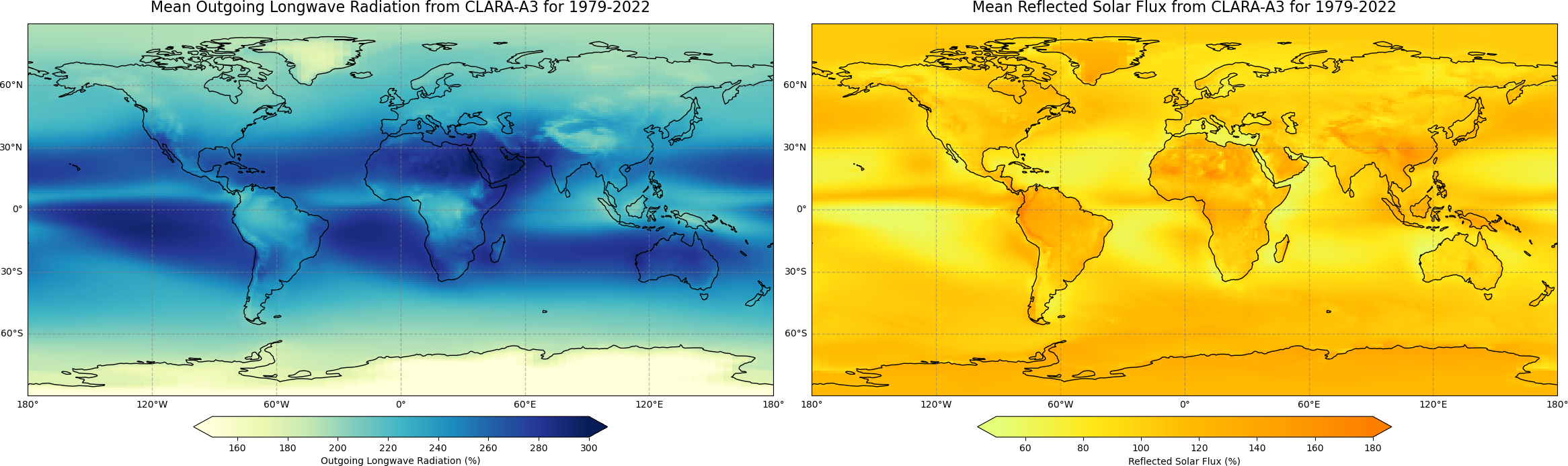
In the following, two examples are presented to illustrate some ideas on the usage, visualisation, and analysis of the CLARA-A3 earth radiation dataset. Two figures below are results of Use Case 1 and 2, and the result of a successful run of the code.
Prepare your environment#
Set up CDSAPI and your credentials#
The code below will ensure that the cdsapi package is installed. If you have not setup your ~/.cdsapirc file with your credenials, you can replace None with your credentials that can be found on the how to api page (you will need to log in to see your credentials).
!pip install -q cdsapi
# If you have already setup your .cdsapirc file you can leave this as None
cdsapi_key = None
cdsapi_url = None
(Install and) Import libraries#
The data have been stored in files written in NetCDF format. To best handle these, we will import the library Xarray which is specifically designed for manipulating multidimensional arrays in the field of geosciences. The libraries Matplotlib and Cartopy will also be imported for plotting and visualising the analysed data. We will also import the libraries zipfile to work with zip-archives, OS to use OS-functions and pattern expansion, and urllib3 for disabling warnings for data download via CDS API.
# CDS API library
import cdsapi

# Libraries for working with multidimensional arrays
import xarray as xr

# Library to work with zip-archives and OS-functions
import zipfile
import os

# Libraries for plotting and visualising data
import matplotlib.pyplot as plt
import cartopy.crs as ccrs

# Disable warnings for data download via API
import urllib3
urllib3.disable_warnings()
Specify data directory#
# Directory to store data
# Please ensure that datadir is a location where you have write permissions
DATADIR = './data_dir/'
# Create this directory if it doesn't exist
os.makedirs(DATADIR, exist_ok=True)
In advance of the following processing and visualisation part we set a directory where to save the figures. Default option is to save figures in the folder:
FIGPATH = '.'# Please ensure that datadir is a location where you have write permissions
Explore data#
The CLARA-A3 dataset is the successor of CLARA-A2.1 and comprises almost 44 years (latest status: 09/2023) of continuous observations of radiation and clouds from space, thereby monitoring their spatial and temporal variability on Earth. Earth Radiation Budget parameters were not included in CLARA-A2.1
The CLARA-A3 radiation dataset contains all surface and Earth (top-of-the-atmosphere) fluxes, and thus, it enables studies of the full earth radiation budget.
Please find further information about the datasets as well as the data in the Climate Data Store sections “Overview”, “Download data” and “Documentation”:
Earth Radiation: Budget https://cds.climate.copernicus.eu/cdsapp#!/dataset/satellite-earth-radiation-budget?tab=overview
Surface Radiation Budget: https://cds.climate.copernicus.eu/cdsapp#!/dataset/satellite-surface-radiation-budget?tab=overview
Cloud Properties: https://cds.climate.copernicus.eu/cdsapp#!/dataset/satellite-cloud-properties?tab=overview
Search for data#
To search for data, visit the CDS website. Here we can search for “Earth Radiation Budget” or simply “ERB” data using the search bar. The data we need for this use case is the Earth’s radiation budget from 1979 to present derived from satellite observations. The Earth Radiation Budget (ERB) comprises the quantification of the reflected radiation from the Sun and the emitted longwave radiation from Earth. This catalogue entry comprises data from a number of sources.
Once you reached the landing page, feel free to have a look at the documentation and information provided.
The data can be found in the “Download data”-tab with a form to select certain variables, years etc. For our use case we select as follows:
Parameters of data to download
Product family:
CLARA-A3 (CM SAF cLoud, Albedo and surface RAdiation dataset from AVHRR data)Origin:
EUMETSAT (European Organisation for the Exploitation of Meteorological Satellites)Variable:
Outgoing longwave radiation (Outgoing LW),Outgoing shortwave radiation (Outgoing SW)Climate data record type:
Thematic Climate Data Record (TCDR)Time aggregation:
Monthly meanYear:
Every year from 1979-2020 (shortcut with "Select all" at the bottom right)Month:
Every month from January to December (shortcut with "Select all" at the bottom right)Geographical area:
Whole available regionFormat:
Zip file (.zip)
At the end of the download form, select “Show API request”. This will reveal a block of code, which you can simply copy and paste into a cell of your Jupyter Notebook (see cell below). Having copied the API request into the cell below, running this will retrieve and download the data you requested into your local directory.
Warning
Please remember to accept the terms and conditions of the dataset, at the bottom of the CDS download form!
Download the data#
With the API request copied into the cells below, running these cells will retrieve and download the data you requested into your local directory.
Note
The download may take a few minutes. Feel free to have a look at the various information on the Earth Radiation Budget page in the CDS or already get familiar with the next steps.
c = cdsapi.Client()

c.retrieve(
    'satellite-earth-radiation-budget',
    {
        'format': 'zip',
        'product_family': 'clara_a3',
        'origin': 'eumetsat',
        'variable': [
            'outgoing_longwave_radiation', 'outgoing_shortwave_radiation',
        ],
        'climate_data_record_type': 'thematic_climate_data_record',
        'time_aggregation': 'monthly_mean',
        'year': ['%04d' % (year) for year in range(1979, 2021)],
        'month': ['%02d' % (mnth) for mnth in range(1, 13)],
    },
    f'{DATADIR}/download_claraA3_erb.zip',
)
2024-12-09 16:13:53,119 INFO [2024-01-09T00:00:00] NOAA/NCEI HIRS OLR was reprocessed from 2007 till 2023. Please see the Known issues section under the Documentation tab for more details.
2024-12-09 16:13:53,121 WARNING [2024-12-09T16:13:53.137329] You are using a deprecated API endpoint. If you are using cdsapi, please upgrade to the latest version.
2024-12-09 16:13:53,121 INFO Request ID is 85037786-023d-424e-b6cf-6ea437e6ab74
2024-12-09 16:13:53,325 INFO status has been updated to accepted
2024-12-09 16:14:08,585 INFO status has been updated to running
2024-12-09 16:22:19,668 INFO status has been updated to successful
'./data/download_claraA3_erb.zip'
The zip-file should be downloaded and saved at the correct place, that we have defined earlier. The zip archive containing one variable for monthly mean needs several GB of storage space.
The following lines unzip the data. DATADIR + ‘/download_claraA3_erb.zip is the path to the zip-file. The first line constructs a ZipFile() object, the second line applies the function extractall to extract the content.
DATADIR/’_ is the path we want to store the files.
with zipfile.ZipFile(DATADIR + '/download_claraA3_erb.zip', 'r') as zip_ref:
    zip_ref.extractall(DATADIR)
With the zip-file unziped and files at the right place we can start reading and processing the data.
Load dataset#
The following line starting with “file” considers only files in the given directory starting the “OLRmm”, “RSFmm” and ending with “.nc” and creates a list with all matching files. The “*” means “everything” and takes every file into account. This is quite useful since year and month are part of the file names.
The second line reads the defined file list with the xarray function “open_mfdataset” (mf - multiple file) and concatenates them according to the time dimension.
file_olr = DATADIR + '/OLRmm*.nc'
file_rsf = DATADIR + '/RSFmm*.nc'

dataset_olr = xr.open_mfdataset(file_olr, concat_dim='time', combine='nested')
dataset_rsf = xr.open_mfdataset(file_rsf, concat_dim='time', combine='nested')
Please find below the xarray dataset of the Earth Radiation Budget exemplary:
It provides information about the:
Dimensions: Lat and Lon with 0.25°x0.25° resolution and a lenght of 720/1440 and 504 months (42 years * 12 months)
Coordinates: Spatial coordinates for Latitude and Longitude, temporal coordinates for time
Data variables: List of different variables (in our case “LW_flux” and “SW_flux” are relevant)
Attributes: Various important information about the dataset
dataset_olr
<xarray.Dataset> Size: 10GB
Dimensions:                   (time: 504, lat: 720, bnds: 2, lon: 1440)
Coordinates:
  * lon                       (lon) float64 12kB -179.9 -179.6 ... 179.6 179.9
  * lat                       (lat) float64 6kB -89.88 -89.62 ... 89.62 89.88
  * time                      (time) datetime64[ns] 4kB 1979-01-01 ... 2020-1...
Dimensions without coordinates: bnds
Data variables:
    lat_bnds                  (time, lat, bnds) float64 6MB dask.array<chunksize=(1, 720, 2), meta=np.ndarray>
    lon_bnds                  (time, lon, bnds) float64 12MB dask.array<chunksize=(1, 1440, 2), meta=np.ndarray>
    time_bnds                 (time, bnds) datetime64[ns] 8kB dask.array<chunksize=(1, 2), meta=np.ndarray>
    record_status             (time) uint8 504B dask.array<chunksize=(1,), meta=np.ndarray>
    number_of_lw_daily_means  (time, lat, lon) float32 2GB dask.array<chunksize=(1, 720, 1440), meta=np.ndarray>
    LW_flux                   (time, lat, lon) float64 4GB dask.array<chunksize=(1, 720, 1440), meta=np.ndarray>
    number_of_lw_inst_obs     (time, lat, lon) float32 2GB dask.array<chunksize=(1, 720, 1440), meta=np.ndarray>
    bitflags_lw               (time, lat, lon) float32 2GB dask.array<chunksize=(1, 720, 1440), meta=np.ndarray>
Attributes: (12/38)
    geospatial_lat_min:         -90.0
    geospatial_lat_max:         90.0
    geospatial_lon_min:         -180.0
    geospatial_lon_max:         180.0
    title:                      CM SAF Cloud, Albedo and Radiation dataset, A...
    summary:                    This file contains AVHRR-based Thematic Clima...
    ...                         ...
    variable_id:                LW_flux
    license:                    The CM SAF data are owned by EUMETSAT and are...
    source:                     FCDR AVHRR-GAC : ERA-5 : OSISAF : USGS : IGBP
    lineage:                    pygac/gac2pps.py : NWC/PPS version v2018 : CL...
    CMSAF_L2_processor:         CLARA-A3 TOA toa_flux v2.0
CMSAF_L3_processor: CLARA-A3 TOA dailymean v2.4Use case 1: the mean global Outgoing Longwave Radiation (OLR) radiation distribution#
Use Case #1 aims to give an overview about the OLR distribution. We do that by plotting the global mean OLR from the CLARA-A3 dataset. Please note that we need to open the dataset to be able to execute this usecase, as described in the previous “Load dataset” section.
Calculation of the temporal average of OLR#
We calculate the temporal average with the function np.nanmean. np is common alias for numpy and a library for mathmatical working with arrays. nanmean averages the data and ignores nan’s. This operation is applied to “dataset_olr” and the variable Outgoing Longwave Radiation or “LW_flux”. axis=0 averages over the first axis, which is “time” in this case. This leads to a two-dimensional result with an average over time.
# Calculate temporal average
average = dataset_olr['LW_flux'].mean(dim="time")

# Get longitude and latitude coordinates. Both are variables of the dataset and available with
# the ".variables['lat/lon']" function; [:] usually means ["from":"till"] but
# without numbers it means "everything"
lon = dataset_olr.variables['lon']
lat = dataset_olr.variables['lat']
Plot of the temporal average of OLR#
With the calculation done the data is ready for a plot. Please find the plot and settings in the next section.
Some further notes:
Matplotlib provides a wide range of colorbars: https://matplotlib.org/stable/users/explain/colors/colormaps.html; the addition
_rreverses the colorbarThe
add_subplotpart provides the option to plot more than one figure (e.g. a 2x2 matrix with four plots together). In this case (1,1,1) means that the panel is a 1x1 matrix and the following plot is the first subplot.
# Create figure and size
fig = plt.figure(figsize=(15, 8))

# Create the figure panel and define the Cartopy map projection (PlateCarree)
ax = fig.add_subplot(1, 1, 1, projection=ccrs.PlateCarree())

# Plot the data and set colorbar, minimum and maximum values
im = plt.pcolormesh(lon, lat, average, cmap='YlGnBu', vmin=150, vmax=300)

# Set title and size
ax.set_title('Mean Outgoing Longwave Radiation from CLARA-A3 for 1979-2020', fontsize=16, pad=12)

# Define gridlines with linewidth, color, opacity and style
gl = ax.gridlines(linewidth=1, color='gray', alpha=0.5, linestyle='--')

# Set x- and y-axis labels to True or False
gl.top_labels = False
gl.bottom_labels = True
gl.left_labels = True

# Set coastlines
ax.coastlines()

# Set colorbar and adjust size, location and text
cbar = plt.colorbar(im, fraction=0.05, pad=0.05, orientation='horizontal', extend='both')
cbar.set_label('Outgoing Longwave Radiation (W/m²)')

# Save figure in defined path and name
plt.savefig(FIGPATH + '/OLRmm_mean.png')

# Show plot and close it afterwards to reduce the amount of storage
plt.show()
plt.close()
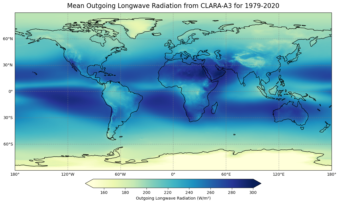
Figure 1 shows the global mean values of the Outgoing Longwave Radiation (OLR).
Use case 2: the mean global Reflected Solar Flux (RSF) distribution#
Use Case #2 aims to give an overview about the RSF distribution. We do that by plotting the global mean RSF from the CLARA-A3 dataset. Please note that we need to open the dataset to be able to execute this usecase, as described in the previous “Load dataset” section.
Calculation of the temporal average of RSF#
We calculate the temporal average with the function np.nanmean. np is common alias for numpy and a library for mathmatical working with arrays. nanmean averages the data and ignores nan’s. This operation is applied to “dataset_olr” and the variable Reflected Solar Flux or “SW_flux”. axis=0 averages over the first axis, which is “time” in this case. This leads to a two-dimensional result with an average over time.
# Calculate temporal average
average = dataset_rsf['SW_flux'].mean(dim="time")

# Get longitude and latitude coordinates. Both are variables of the dataset and available with
# the ".variables['lat/lon']" function; [:] usually means ["from":"till"] but
# without numbers it means "everything"
lon = dataset_rsf.variables['lon']
lat = dataset_rsf.variables['lat']
Plot of the temporal average of RSF#
With the calculation done the data is ready for a plot. Please find the plot and settings in the next section.
# Create figure and size
fig = plt.figure(figsize=(15, 8))

# Create the figure panel and define the Cartopy map projection (PlateCarree)
ax = fig.add_subplot(1, 1, 1, projection=ccrs.PlateCarree())

# Plot the data and set colorbar, minimum and maximum values
im = plt.pcolormesh(lon, lat, average, cmap='Wistia_r', vmin=50, vmax=200)

# Set title and size
ax.set_title('Mean Reflected Solar Flux from CLARA-A3 for 1979-2020', fontsize=16, pad=12)

# Define gridlines with linewidth, color, opacity and style
gl = ax.gridlines(linewidth=1, color='gray', alpha=0.5, linestyle='--')

# Set x- and y-axis labels to True or False
gl.top_labels = False
gl.bottom_labels = True
gl.left_labels = True

# Set coastlines
ax.coastlines()

# Set colorbar and adjust size, location and text
cbar = plt.colorbar(im, fraction=0.05, pad=0.05, orientation='horizontal', extend='both')
cbar.set_label('Reflected Solar Flux (W/m²)')

# Save figure in defined path and name
plt.savefig(FIGPATH + '/RSFmm_mean.png')

# Show plot and close it afterwards to reduce the amount of storage
plt.show()
plt.close()
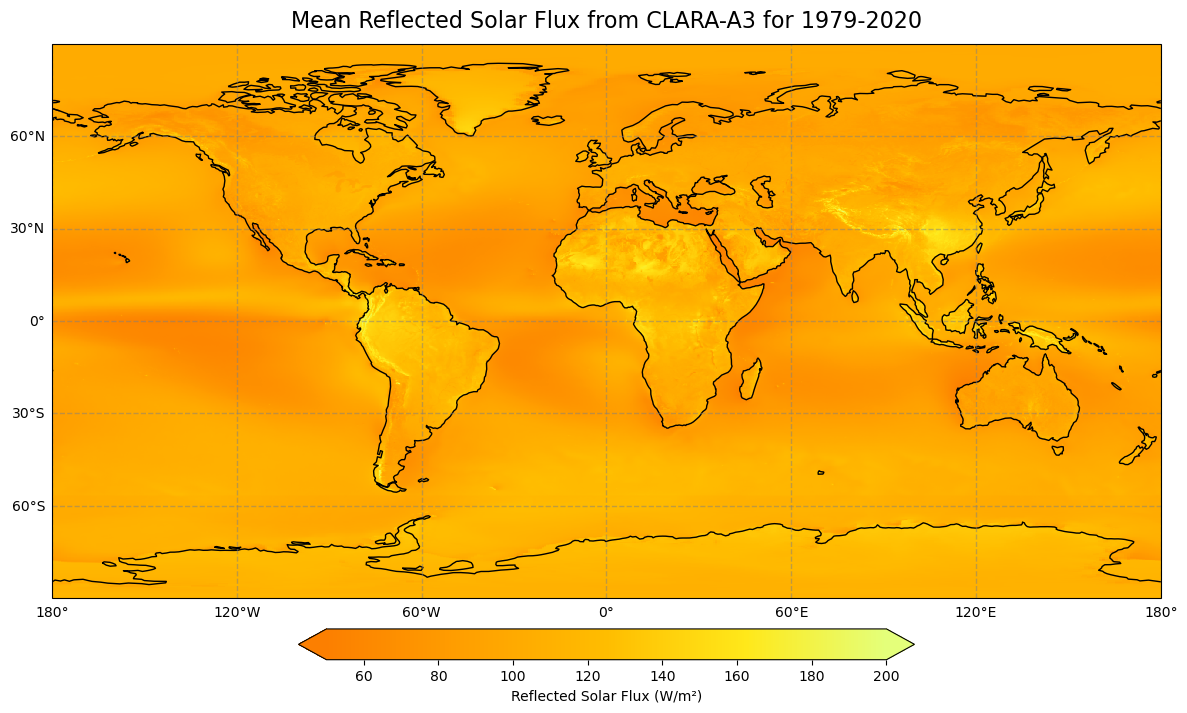
Figure 2 shows the global mean values of the Reflected Solar Flux (RSF).