Michael Buchwitz, 20-Nov-2024

How to access, read and use satellite XCO2 and XCH4 Level 3 data products#
This notebook can be run on free online platforms, such as Binder, Kaggle and Colab, or they can be accessed from GitHub. The links to run this notebook in these environments are provided here, but please note they are not supported by ECMWF.
![]()

![]()
Introduction#
Several satellite-derived Essential Climate Variable (ECV) atmospheric data products are generated for GHGs (\(CO_2\) and \(CH_4\)), aerosols and ozone. This Jupyter Notebook (JN) focusses on GHG Level 3 (L3) products. The other products are covered by separate JNs. The GHG L3 products are available at a spatial resolution of 5 deg latitude times 5 deg longitude and monthly time resolution. In contrast, Level 2 (L2) products contain retrieved parameters for individual satellite ground pixels (footprints). How to use L2 GHG products is described in a separate JN.
The GHG L3 products contain column-averaged dry-air mole fractions of \(CO_2\) and \(CH_4\), denoted XCO2 (in parts per million - ppm) and XCH4 (in parts per billion - ppb). They are derived from SCIAMACHY/ENVISAT, GOSAT, GOSAT-2 and OCO-2. The relevant peer-reviewed publication describing the algorithm and an earlier version of the data products is Reuter et al., 2020 (https://amt.copernicus.org/articles/13/789/2020/). The relevant technical documentation and further information is available on the CDS website (https://cds.climate.copernicus.eu/).
Learning objectives 🎯#
This Jupyter Notebook (JN) illustrates how to access, read and use Greenhouse Gas (GHG) atmospheric carbon dioxide (\(CO_2\)) and methane (\(CH_4\)) data products as generated in the framework of the Copernicus Climate Change Service (C3S).
The atmospheric concentration of both gases varies in time and in space. This JN focusses on two use cases.
The first use case is related to temporal variations. Temporal atmospheric concentration variations depend, for example, on latitude. Seasonal variations are, for example, different for the northern hemisphere (NH) and the southern hemisphere (SN), whereas the increasing trend is similar for different latitude bands. This can be investigated by generating and plotting time series for latitude bands. How this can be done is shown in this JN.
The second use case is related to spatial variations. Here it is shown how spatial maps of GHG concentrations and their uncertainty can be generated. Depending on time (month, season) XCO2 maps show large differences of the \(CO_2\) concentration in the two hemispheres, i.e., a significant interhemispheric \(CO_2\) gradient. This is also observed for XCH4. In each hemisphere the concentration of both gases is quite similar as both gases are long lived and well mixed due to atmospheric transport and diffusion. Nevertheless, strong source regions are sometimes (during certain months) directly visible via locally enhanced concentrations. This can be seen and investigated by generating monthly XCO2 and XCH4 maps. The monthly maps also show the time dependent spatial coverage of the satellite-derived data products. This is primarily due to the fact that these satellite observations require good solar illumination conditions. The spatial coverage therefore closely follows the sun with better coverage of the summer hemisphere compared to the winter hemisphere. Data gaps are also due to clouds (all data are filtered to avoid cloud contamination), water surfaces (oceans and lakes, etc., are poor reflectors of solar radiation in the short-wave infra-red spectral range except for sun-glint observing conditions) and for other reasons. How these spatial maps can be generated is shown in this JN.
Prepare your environment#
Before we begin we must prepare our environment. This includes installing the Application Programming Interface (API) of the CDS, and importing the various python libraries that we will need.
Set up CDSAPI and your credentials#
The code below will ensure that the cdsapi package is installed. If you have not setup your ~/.cdsapirc file with your credentials, you can replace None with your credentials that can be found on the how to api page (you will need to log in to see your credentials).
!pip install -q cdsapi
# If you have already setup your .cdsapirc file you can leave this as None
cdsapi_key = None
cdsapi_url = None
(Install and) Import libraries#
First we have to import some modules:
# Import libraries needed for the Jupyter notebook

# Note that lines starting with "#" are comment lines

# Libraries for working with data, especially multidimensional arrays
import numpy as np
import pandas as pd
import xarray as xr

# Library to work with zip-archives, operating system (OS) functions and pattern expansion
import zipfile
import os
from pathlib import Path

# Libraries for plotting and visualising data
import matplotlib.pyplot as plt
import matplotlib as mplt
#import matplotlib.dates as md
import cartopy.crs as ccrs
import datetime

# Libraries for style parameters
from pylab import rcParams
import seaborn as sns

# Disable warnings for data download via API
import urllib3
urllib3.disable_warnings()

print('* ... finished importing modules')
* ... finished importing modules
Specify data directory#
# Specify local data directory for the downloads:

#data_directory = "./data_dir_tmp/"   # Test only
data_directory = "data_dir"

DATADIR = Path(data_directory)

if not os.path.exists(DATADIR):
   print('* Generating: ', DATADIR)
   os.mkdir(DATADIR)
else:
   print('* sub-directory exists: ', DATADIR)
* sub-directory exists: data_dir
Explore data#
The C3S GHG data products used here are retrieved from satellite radiance measurement using dedicated retrieval algorithms. Most of these algorithms have been developed in the past within the Climate Change Initiative (CCI) of the European Space Agency (ESA). These algorithms are now used to operationally generate the corresponding data products within the European Union (EU) C3S project. The data products are freely available for all interested users from the Copernicus Climate Data Store (CDS, https://cds.climate.copernicus.eu/).
The L3 XCO2 data product used here has product identifier (ID) XCO2_OBS4MIPS and the L3 XCH4 product ID is XCH4_OBS4MIPS. The code has been tested using version 4.5 of these products, which covers the period from beginning of 2003 to end of 2022.
The C3S GHG data products and their documentation are available from the CDS website.
\(CO_2\) data and documents are available from https://cds.climate.copernicus.eu/datasets/satellite-carbon-dioxide?tab=overview.
\(CH_4\) data and documents are available from https://cds.climate.copernicus.eu/datasets/satellite-methane?tab=overview.
Each satellite-derived \(CO_2\) or \(CH_4\) data product as generated in C3S and made available via the CDS has a unique product ID. The product IDs of the Level 3 products used here are XCO2_OBS4MIPS and XCH4_OBS4MIPS. Each products consists of a single NetCDF file in Obs4MIPs format (https://esgf-node.llnl.gov/projects/obs4mips/). These products have been generated by merging data products from different satellite sensors. On the CDS website these products can be selected and downloaded by selecting “MERGED and OBS4MIPS” for item “Sensor and algorithm” as described in details in the following section.
Search for the data#
In the following we explain how to obtain XCO2_OBS4MIPS v4.5 data product files.
The same method can be used to get the corresponding methane product XCH4_OBS4MIPS or another version of these Level 3 products.
Visit the CDS website https://cds.climate.copernicus.eu/ and search for “CO2” in the search field.
Then click on: Carbon dioxide data from 2002 to present derived from satellite observations
Select the desired product by choosing the parameters you are interested from the “Download” tab:
Parameters of data to download
Processing level:
Level 3Variable:
Column-average dry-air mole fraction of atmospheric Carbon Dioxide (XCO2) and related variablesSensor and algorithm:
MERGED and OBS4MIPSVersion:
4.5
At the end of the download form, select “Show API request”. This will reveal a block of code, which you can simply copy and paste into a cell of your Jupyter Notebook (see cell below). Having copied the API request into the cell below, running this will retrieve and download the data you requested into your local directory.
Warning
Please remember to accept the terms and conditions of the dataset, at the bottom of the CDS download form!
Setting default plot style parameters#
# The following style parameters will be used for all plots in this use case.
rcParams['figure.figsize'] = [15,5]
rcParams['figure.dpi'] = 350
#rcParams['font.family'] = 'serif'
rcParams['font.family'] = 'Arial'
#rcParams['font.serif'] = mplt.rcParamsDefault['font.serif']
#rcParams['mathtext.rm'] = 'serif:light'
#rcParams['mathtext.it'] = 'serif:italic'
#rcParams['mathtext.bf'] = 'serif:bold'
rcParams['mathtext.default'] = 'regular'
plt.rc('font', size=17)          # controls default text sizes
plt.rc('axes', titlesize=17)     # fontsize of the axes title
plt.rc('axes', labelsize=17)     # fontsize of the x and y labelsize
plt.rc('xtick', labelsize=15)    # fontsize of the tick labels
plt.rc('ytick', labelsize=15)    # fontsize of the tick labels
plt.rc('legend', fontsize=10)    # fontsize of the legend
plt.rc('figure', titlesize=18)   # fontsize of the figure title

projection = ccrs.PlateCarree()
mplt.rc('xtick', labelsize=9)
mplt.rc('ytick', labelsize=9)

print('* ... finished setting default plot style parameters')
* ... finished setting default plot style parameters
Product selection: XCO2 or XCH4 Level 3 OBS4MIPS product#
Select the desired product by activating either the line with XCO2 or the line with XCH4. Here we have selected XCH4:
# Select one main product (by commenting in/out):
#product_name = 'XCO2'
product_name = 'XCH4'

product_id = product_name+'_OBS4MIPS'

#Select product version (by commenting in / out):
#product_version = 'v4.4'; product_version_str2 = '4_4'; product_period = '200301_202112'
product_version = 'v4.5'; product_version_str2 = '4_5'; product_period = '200301_202212'

print('* Selected Level 3 product:')
print('* product_id: ', product_id)
print('* product_version: ', product_version)
* Selected Level 3 product:
* product_id:  XCH4_OBS4MIPS
* product_version:  v4.5
Product specific settings#
Here some variables are set depending on the selected product:
# Define some product specific variables:
if product_name == 'XCO2':
   wanted_variable      = 'xco2'        # main variable
   wanted_variable_unc  = 'xco2_stderr' # uncertainty of main variable
   unit_conv         = 1e6              # unit conversion factor from mole/mole to ppm
   unit              = '[ppm]'          # desired unit
if product_name == 'XCH4':
   wanted_variable      = 'xch4'        # main variable
   wanted_variable_unc  = 'xch4_stderr' # uncertainty of main variable
   unit_conv         = 1e9              # unit conversion factor from mole/mole to ppb
   unit              = '[ppb]'          # desired unit

print('* wanted_variable: ', wanted_variable)
* wanted_variable: xch4
Download the data#
# Have the data already been downloaded (please select by commenting in/out)?:
product_already_downloaded = 'no'     # Default
#product_already_downloaded = 'yes'   # Use this if data already downloaded

if product_already_downloaded == 'no':

   print('* downloading product ...')

   # Code obtained via "Show API request code" (see above):

   if product_name == 'XCO2':
      # Copy code obtained from "Show API request code":
      import cdsapi
      dataset = "satellite-carbon-dioxide"
      request = {
         "processing_level": ["level_3"],
          "variable": "xco2",
          "sensor_and_algorithm": "merged_obs4mips",
          #"version": ["4_5"]
          "version": [product_version_str2]
      }

   if product_name == 'XCH4':
      # Copy code obtained from "Show API request code":
      import cdsapi
      dataset = "satellite-methane"
      request = {
         "processing_level": ["level_3"],
          "variable": "xch4",
          "sensor_and_algorithm": "merged_obs4mips",
          #"version": ["4_5"]
          "version": [product_version_str2]
      }

   client = cdsapi.Client(url=cdsapi_url, key=cdsapi_key)
   # Generates download.zip file in current directory:
   client.retrieve(dataset, request).download('download.zip')

   # Unzip:
   path_to_zip_file        = 'download.zip'
   with zipfile.ZipFile(path_to_zip_file, 'r') as zip_ref:
    zip_ref.extractall(DATADIR)

else:
    print('* The following has been selected: product_already_downloaded: ', product_already_downloaded)
    print('* Therefore, no data download via cdsapi')
* downloading product ...
2025-10-14 17:40:38,176 INFO Request ID is 4c23dc5e-c30c-40ba-a089-5d8fe6370880
2025-10-14 17:40:38,276 INFO status has been updated to accepted
2025-10-14 17:40:46,802 INFO status has been updated to running
2025-10-14 17:40:51,940 INFO status has been updated to successful
Inspect data#
# If the above cell has been executed for both products, then following two files should be located in sub-directory data_dir:
# 200301_202212-C3S-L3_XCO2-GHG_PRODUCTS-MERGED-MERGED-OBS4MIPS-MERGED-v4.5.nc
# 200301_202212-C3S-L3_XCH4-GHG_PRODUCTS-MERGED-MERGED-OBS4MIPS-MERGED-v4.5.nc

# Check if the desired file exists:
wanted_file_OK = 'no'
wanted_file = product_period+'-C3S-L3_'+product_name+'-GHG_PRODUCTS-MERGED-MERGED-OBS4MIPS-MERGED-'+product_version+'.nc'
wanted_path_file = DATADIR/wanted_file
print('* wanted product file: ', wanted_path_file)
if (os.path.exists(wanted_path_file) == True):
   print('* ... file exists')
   wanted_file_OK = 'yes'
else:
   print('* ERROR: File does not exist !?')
* wanted product file:  data_dir/200301_202212-C3S-L3_XCH4-GHG_PRODUCTS-MERGED-MERGED-OBS4MIPS-MERGED-v4.5.nc
* ... file exists
Reading the OBS4MIPS file#
Open and read the data file:
if wanted_file_OK == 'yes':
   print('* reading: ', wanted_path_file)
   ds = xr.open_dataset(wanted_path_file)                    # Read data
   product_version_2 = ds.attrs['source_version_number']     # Get version number
   n_time = ds.dims['time']                                  # Get number of times = number of months
   gas = ds[wanted_variable] * unit_conv                     # conversion to ppm or ppb
   land_fraction = ds["land_fraction"]                       # land fraction (0.0 = 0% land (=100% water); 1.0 = 100% land)
else:
   print('* ERROR: File does not exist !?')
* reading: data_dir/200301_202212-C3S-L3_XCH4-GHG_PRODUCTS-MERGED-MERGED-OBS4MIPS-MERGED-v4.5.nc
/var/folders/kx/ksg5wbrj1sq95rp2tz_72j6c0000gn/T/ipykernel_8121/4059709852.py:5: FutureWarning: The return type of `Dataset.dims` will be changed to return a set of dimension names in future, in order to be more consistent with `DataArray.dims`. To access a mapping from dimension names to lengths, please use `Dataset.sizes`.
  n_time = ds.dims['time']                                  # Get number of times = number of months
Application 1: Investigating time series for selected latitude band#
Here the user can select a latitude band by specifying the variables lat_min and lat_max.
For this latitude band, the data covering the entire time series are generated and plotted.
if wanted_file_OK == 'yes':
   print('* generating time series for latitude band ...')
   lat_min = 30.0; lat_max = '60.0'; land_fraction_min = 0.95; lat_band_str = 'Northern Mid-latitudes (30N - 60N), land' # Define latitude band
   #gas_lat_band = gas.sel(lat=slice(lat_min,lat_max))                            # Get data for latitude band
   gas_lat_band           = gas.sel(lat=slice(lat_min, lat_max))                  # Get data for latitude band
   land_fraction_lat_band = land_fraction.sel(lat=slice(lat_min, lat_max))        # Get land fractions for latitude band
   (idx_not_land) = (land_fraction_lat_band.values < land_fraction_min).nonzero() # Get indices of non-land grid cells
   s_fyear  = []   # list for fractional year
   s_year   = []   # year
   s_month  = []   # month
   s_gas    = []   # mean value of gas (i.e., XCO2 or XCH4) in latitude band
   for ii in range(n_time):                           # loop over all months
      act_time     = gas.time.values[ii]              # get time
      act_time_str = str(act_time)                    # convert time to string
      act_year     = int(act_time_str[0:4])           # get year
      act_month    = int(act_time_str[5:7])           # get month
      act_fyear    = act_year + (act_month-0.5)/12.0  # get fractional year
      tmp_gas      = gas_lat_band.isel(time=ii)       # get all gas values in latitude band for act. month
      tmp_gas[(idx_not_land)] = np.nan                # Set non-land cells to NaN
      act_gas      = tmp_gas.mean(skipna=True).values # get gas mean value for act. month
      if (np.isnan(act_gas) == False):
         #print('* ii act_time act_gas: ', ii, act_time, act_gas)
         s_fyear.append(act_fyear)         # fractional year
         s_year.append(act_year)
         s_month.append(act_month)
         s_gas.append(act_gas)
      #else:
      #   print('* Warning: gas value is NaN for year month: ', act_year, act_month)
      #   if ((act_year == 2015) & (act_month == 1)):
      #      print('* Note: No satellite data available for January 2015')
   s_fyear  = np.array(s_fyear)
   s_year   = np.array(s_year)
   s_month  = np.array(s_month)
   s_gas    = np.array(s_gas)                      # land fraction (0.0 = 0% land (=100% water); 1.0 = 100% land)
else:
   print('* ERROR: File does not exist !?')
* generating time series for latitude band ...
Plotting time series#
if wanted_file_OK == 'yes':
   # Plot time series:
   print('* plotting time series ...')
   sns.set()                             # select seaborn for plot style
   figsize = (8,5)
   fig = plt.figure(figsize=figsize)     # page size
   pos = [0.12, 0.14, 0.85, 0.80]        # position (left,bottom,width,height) in page coord
   ax  = fig.add_axes(pos)
   ax.ticklabel_format(useOffset=False)  # prevent scientific notation axis numbering
   xmin = np.min(s_year)                 # x axis range and annotation
   xmax = np.max(s_year)+1
   xxx_int = np.arange(xmin, xmax, 2)
   xxx_ano = [str(x) for x in xxx_int]
   ax.set_xticks(xxx_int)
   #ax.set_xticklabels(xxx_ano, fontsize=12)
   ax.set_xticklabels(xxx_ano)
   rmin = np.min(s_gas)*0.99             # y axis range
   rmax = np.max(s_gas)*1.01
   title = product_id+' '+product_version_2
   xtitle = 'Time [year]'
   ytitle = product_name+' '+unit
   plt.scatter(s_fyear, s_gas, s=3, zorder=10, color='blue')
   plt.plot(s_fyear, s_gas, zorder=10, color='blue', label=lat_band_str)
   ymin = rmin; ymax = rmax
   plt.axis([xmin, xmax, ymin, ymax])
   plt.title(title, fontsize=12); plt.xlabel(xtitle); plt.ylabel(ytitle)
   plt.legend(loc='upper left', fontsize='medium')
   plot_type = 'png'
   if plot_type == 'png':
      o_file_plot = product_id+'_'+product_version+'_timeseries.png'
      print('* generating: ', o_file_plot)
      plt.savefig(o_file_plot, dpi=600)
   else:
      plt.show()
else:
    print('* ERROR: File does not exist !?')
* plotting time series ...
* generating:  XCH4_OBS4MIPS_v4.5_timeseries.png
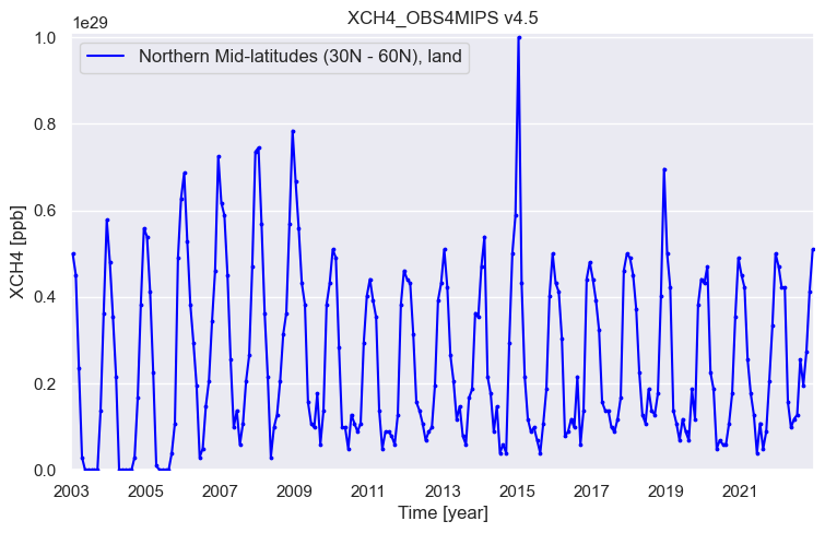
What does this time series tells us? As can be seen, XCH4 has a strong seasonal cycle with a maximum in the second half of each year over northern hemispheric mid-latitudes. This is mainly due to natural sources such as wetlands, where \(CH_4\) emissions are largest when temperatures are high. As can also be seen, XCH4 was (apart from seasonal fluctuations) relatively constant until about 2006. Since 2007 methane is increasing (increasing again as methane was also increasing for several decades until the late 1990th). Additional information on these satellite-derived XCH4 and XCO2 time series can be found in the Copernicus press release from January 2023, where an earlier version of this data sets have been used: “Copernicus: 2022 was a year of climate extremes, with record high temperatures and rising concentrations of greenhouse gases”, see https://climate.copernicus.eu/copernicus-2022-was-year-climate-extremes-record-high-temperatures-and-rising-concentrations. Please have to look at that website to get additional information about the evolution of atmospheric CO2 and XCH using these satellite observations including links to relevant scientific publications.
Application 2: Investigating spatial variations and coverage#
Here the user can chose time (year and month) and spatial domain to generate plots of the spatial distribution of the selected GHG.
if wanted_file_OK == 'yes':
   print('* plotting map ...')

   # Select year and month:
   wanted_year  = '2021'
   wanted_month = '09'

   # Get (only) data for wanted month
   wanted_time = wanted_year+'-'+wanted_month
   da = ds.sel(time=wanted_time)
   n_time_da = da.dims['time']
   plot_map_OK = 'no'
   #print('* n_time_da (should be 1 (= 1 month) !?): ', n_time_da)
   if n_time_da != 1:
      print('* ERROR: n_time_da != 1: ', n_time_da)
   else:
      # Get lat, lon, data for plot
      coord_lat  = da.coords['lat'].values          # Get latitudes
      coord_lon  = da.coords['lon'].values          # Get longitudes
      data = da[wanted_variable]                    # Get xco2 or xch4
      act_time = data.time.values[0]                # Get time
      ts = pd.to_datetime(str(act_time))
      act_year  = ts.strftime('%Y')
      act_month = ts.strftime('%m')
      data = data.isel(time=0)                      # Remove time dimension
      data = data * unit_conv                       # conversion to ppm or ppb
      plt_data     = data.values                    # Get data values to be plotted
      plt_data_min = float(data.min().values)         # Get minimum data value for plot
      plt_data_max = float(data.max().values)         # Get maximum data value for plot
      plt_data_mean     = np.nanmean(plt_data)      # Compute mean value
      plt_data_std      = np.nanstd(plt_data)       # Compute standard deviation
      plt_data_mean_str = '{:.1f}'.format(plt_data_mean)
      plt_data_std_str  = '{:.1f}'.format(plt_data_std)
      plt_data_str      = 'mean+/-std: '+plt_data_mean_str+'+/-'+plt_data_std_str
      # ------------------
      plt_lat      = coord_lat
      plt_lon      = coord_lon
      sns.set()                                     # use seaborn plot style
      proj = ccrs.PlateCarree()
      latlon_bounds = [-180, 180, -90, 90]          # Set lat/lon range for plot
      figsize = (8,5)                               # Figure size
      # -------
      n_ticks = 5                                   # Set color bar parameters
      vmin  = plt_data_min
      vmax  = plt_data_max
      vinc  = (vmax-vmin) / n_ticks
      vinc  = float(np.ceil(vinc)) # next largest int
      vmax  = vmin + n_ticks * vinc
      # -------
      fig = plt.figure(figsize=figsize) # page size
      pos = [0.08, 0.22, 0.84, 0.72] # position (left,bottom,width,height) in page coordinates
      ax  = fig.add_axes(pos, projection=proj)
      cs = ax.pcolormesh(plt_lon, plt_lat, plt_data, shading='auto', cmap='viridis', transform=proj, vmin=vmin, vmax=vmax)
      ax.coastlines()
      drawmeridians_label = True
      gl = ax.gridlines(crs=proj, draw_labels=drawmeridians_label, linewidth=1, color='gray', alpha=0.2)
      gl.top_labels  = False
      tit = product_id+' '+product_version_2+' '+wanted_year+wanted_month+': Variable = '+wanted_variable
      ax.set_title(tit, fontsize=15)
      # color bar:
      cbar_ax        = fig.add_axes([0.3, 0.14, 0.4, 0.03]) # position
      cbar           = fig.colorbar(cs, cax=cbar_ax, ticks=np.arange(vmin, vmax, vinc), orientation='horizontal', extend='both')
      cbar_title     = wanted_variable+' '+unit
      cbar.set_label(cbar_title, rotation=0, fontsize=11, labelpad=5) # labepad->y-shift
      # ----------------------------------------
      plot_map_OK = 'yes'
      # ----------------------------------------
      plot_type = 'png'
      if plot_type == 'png':
         o_file_plot = product_id+'_'+product_version+'_map_main.png'
         print('* generating: ', o_file_plot)
         plt.savefig(o_file_plot, dpi=600)
      else:
         plt.show()
* plotting map ...
* generating:  XCH4_OBS4MIPS_v4.5_map_main.png
/var/folders/kx/ksg5wbrj1sq95rp2tz_72j6c0000gn/T/ipykernel_8121/3272796311.py:11: FutureWarning: The return type of `Dataset.dims` will be changed to return a set of dimension names in future, in order to be more consistent with `DataArray.dims`. To access a mapping from dimension names to lengths, please use `Dataset.sizes`.
  n_time_da = da.dims['time']
/Library/Frameworks/Python.framework/Versions/3.12/lib/python3.12/site-packages/numpy/lib/_nanfunctions_impl.py:1872: RuntimeWarning: overflow encountered in multiply
  sqr = np.multiply(arr, arr, out=arr, where=where)
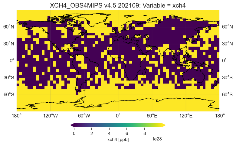
As can be seen, the spatial variation is typically small. The largest difference is often the inte-hemispheric difference, i.e., the concentration difference between the two hemispheres. Nevertheless, strong source regions may be visible via locally enhanced concentrations.
Here a second maps is generated to see the corresponding (1-sigma) uncertainty of the satellite observations, which is contained for each month and each grid cell in the data product.
if wanted_file_OK == 'yes':
   print('* plotting 2nd map (uncertainty) ...')
   if plot_map_OK != 'yes':
      print('* ERROR: Cannot plot uncertainty map: plot_map_OK: ', plot_map_OK)
   else:
      data_unc = da[wanted_variable_unc]      # Get xco2 or xch4 uncertainty
      data_unc = data_unc.isel(time=0)        # Remove time dimension
      data_unc = data_unc * unit_conv         # conversion to ppm or ppb
      plt_data_unc     = data_unc.values  #
      plt_data_unc_min = float(data_unc.min().values)
      plt_data_unc_max = float(data_unc.max().values)
      plt_data_unc_mean     = np.nanmean(plt_data_unc)
      plt_data_unc_std      = np.nanstd(plt_data_unc)
      plt_data_unc_mean_str = '{:.1f}'.format(plt_data_unc_mean)
      plt_data_unc_std_str  = '{:.1f}'.format(plt_data_unc_std)
      plt_data_unc_str      = 'mean+/-std: '+plt_data_unc_mean_str+'+/-'+plt_data_unc_std_str
      # ------------------
      # -------
      n_ticks = 5                            # Set color bar parameters
      vmin  = 0
      vmax  = plt_data_unc_max
      vinc  = (vmax-vmin) / n_ticks
      vinc  = float(np.ceil(vinc))             # next largest int
      vmax  = vmin + n_ticks * vinc
      # -------
      figsize = (8,5)                        # figure size
      pos = [0.08, 0.22, 0.84, 0.72]         # position (left,bottom,width,height) in page coordinates
      fig2 = plt.figure(figsize=figsize)
      ax2  = fig2.add_axes(pos, projection=proj)
      cs = ax2.pcolormesh(plt_lon, plt_lat, plt_data_unc, shading='auto', cmap='viridis', transform=proj, vmin=vmin, vmax=vmax)
      ax2.coastlines()
      gl = ax2.gridlines(crs=proj, draw_labels=drawmeridians_label, linewidth=1, color='gray', alpha=0.2)
      gl.top_labels  = False
      tit = product_id+' '+product_version_2+' '+wanted_year+wanted_month+': Variable = '+wanted_variable_unc
      ax2.set_title(tit, fontsize=15)
      # color bar:
      cbar_ax        = fig2.add_axes([0.3, 0.14, 0.4, 0.03]) # position
      cbar           = fig2.colorbar(cs, cax=cbar_ax, ticks=np.arange(vmin, vmax, vinc), orientation='horizontal', extend='both')
      cbar_title     = wanted_variable_unc+' '+unit
      cbar.set_label(cbar_title, rotation=0, fontsize=11, labelpad=5) # labepad->y-shift
      # ----------------------------------------
      plot_type = 'png'
      if plot_type == 'png':
         o_file_plot = product_id+'_'+product_version+'_map_unc.png'
         print('* generating: ', o_file_plot)
         plt.savefig(o_file_plot, dpi=600)
      else:
         plt.show()
* plotting 2nd map (uncertainty) ...
* generating:  XCH4_OBS4MIPS_v4.5_map_unc.png
/Library/Frameworks/Python.framework/Versions/3.12/lib/python3.12/site-packages/numpy/lib/_nanfunctions_impl.py:1872: RuntimeWarning: overflow encountered in multiply
  sqr = np.multiply(arr, arr, out=arr, where=where)
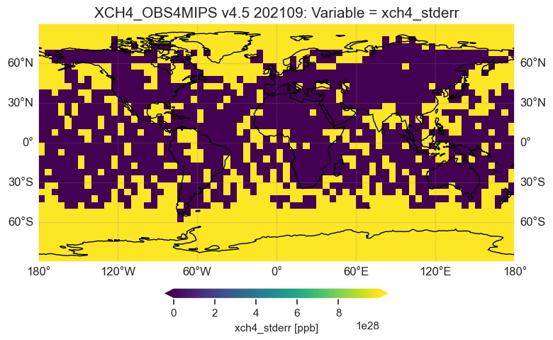
As can be seen, the uncertainty is similar for most regions. For XCH4 the uncertainty is typically on the order of 10 ppb, but may be as large a 20 or 30 ppb for some regions. These are mostly regions with sparse coverage (e.g. due to clouds) and/or a poorly reflecting surface.