CARRA2 temperature forecast - Jupyterbook template

In this notebook we demonstrate how to download a forecast timeseries from CARRA2

Load dependencies and create folders¶

In the first cell we load the relevant libraries for this notebook We also create folders for downloaded data and plots if we want to save them

import cartopy.crs as ccrs
import cartopy.feature as cfeature
import cdsapi
import cfgrib
import matplotlib.path as mpath
import matplotlib.pyplot as plt
import numpy as np
import os
import xarray as xr

Download fields¶

In the section below, fields are downloaded and stored. We will look at temperature of June 2nd, 2024. The resulting data file size is roughly 500 Mb.

target_path = os.path.join('data', 'temperature_timeseries.grib')


dataset = "reanalysis-pan-carra"
request = {
    "level_type": "single_levels",
    "variable": ["2m_temperature"],
    "product_type": "forecast",
    "time": ["00:00", "12:00"],
    "leadtime_hour": [
        "1",
        "2",
        "3",
        "4",
        "5",
        "6",
        "7",
        "8",
        "9",
        "10",
        "11",
        "12",
        "13",
        "14",
        "15",
        "16",
        "17",
        "18"
    ],
    "year": ["2024"],
    "month": ["06"],
    "day": ["02"],
    "data_format": "grib"
}

client = cdsapi.Client()
client.retrieve(dataset, request).download(target_path)

ds = cfgrib.open_dataset(target_path)
ds

Plot a timeseries of temperature¶

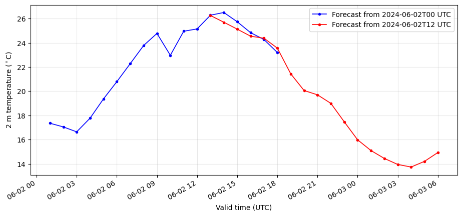
We now plot the temperature over a coordinate in Denmark. Notice the overlapping period between the two forecasts.

target_lat = 55.65
target_lon = 12.45

lat2d = ds["latitude"].values
lon2d = ((ds["longitude"].values + 180) % 360) - 180 
dist = (lat2d - target_lat) ** 2 + (lon2d - target_lon) ** 2
iy, ix = np.unravel_index(np.argmin(dist), dist.shape)
print(f"Nearest grid point coordinates: lat={lat2d[iy, ix]:.3f}, lon={lon2d[iy, ix]:.3f}")

point = ds["t2m"].isel(y=iy, x=ix) - 273.15

colors = ["blue", "red"]
fig, ax = plt.subplots(figsize=(11, 5))
for i in range(ds.sizes["time"]):
    run_time = np.datetime64(ds["time"].values[i], "h")
    ax.plot(ds["valid_time"].values[i], point.isel(time=i).values,
            marker="o", ms=3, lw=1.2, color=colors[i],
            label=f"Forecast from {str(run_time)} UTC")
ax.set_xlabel("Valid time (UTC)")
ax.set_ylabel("2 m temperature ($^\\circ$C)")
ax.legend()
ax.grid(True, alpha=0.3)
fig.autofmt_xdate()

fig.savefig(os.path.join("plots", "temperature_timeseries.png"),
            dpi=150, bbox_inches="tight")
plt.show()

Nearest grid point coordinates: lat=55.661, lon=12.448