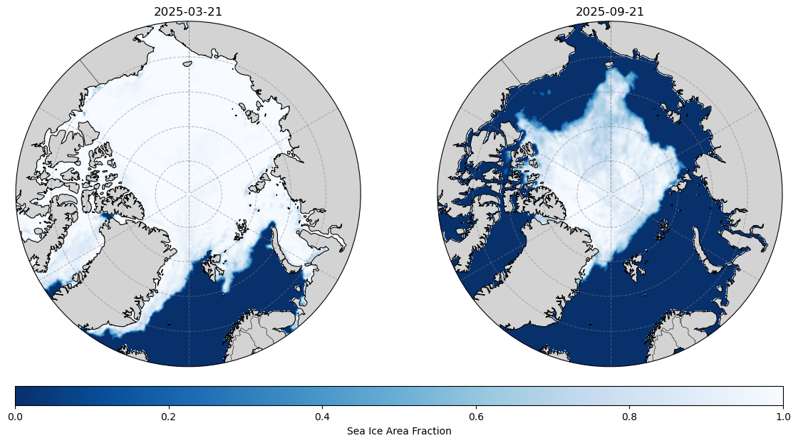
Retrieve and plot sea ice concentration

This notebook demonstrates how to download daily mean values of sea ice concentration for two dates. This example uses the native grib2 format of CARRA2

Load dependencies and create folders¶

In the first cell we load the relevant libraries for this notebook and create folders for downloads and plots

import cartopy.crs as ccrs
import cartopy.feature as cfeature
import cdsapi
import cfgrib
import matplotlib.path as mpath
import matplotlib.pyplot as plt
import numpy as np
import os
import xarray as xr

os.makedirs('data', exist_ok=True)
os.makedirs('plots', exist_ok=True)

Download fields¶

In the section below, fields are downloaded and stored. The resulting data file is roughly 5Mb.

target_path = os.path.join('data', 'sea_ice_area_fraction.grib')

dataset = "reanalysis-pan-carra-means"
request = {
    "time_aggregation": "daily",
    "level_type": "single_levels",
    "variable": ["sea_ice_area_fraction"],
    "product_type": "analysis_based",
    "year": ["2025"],
    "month": ["03", "09"],
    "day": ["21"],
    "data_format": "grib"
}

client = cdsapi.Client()
client.retrieve(dataset, request).download(target_path)

Load and inspect dataset¶

Having downloaded the selected dates as a grib2 file, we can now open it as an xarray dataset using cfgrib

ds = xr.open_dataset(target_path, engine='cfgrib')
ds

Plot snapshots of sea ice minimum and maximum¶

Upon inspection, we can now plot the sea ice cover for the two dates. We define a circular boundary for aesthetics.

fig, axes = plt.subplots(1, 2, figsize=(14, 7), subplot_kw={'projection': ccrs.NorthPolarStereo()})
theta = np.linspace(0, 2*np.pi, 100)
center, radius = [0.5, 0.5], 0.5
verts = np.vstack([np.sin(theta), np.cos(theta)]).T
circle = mpath.Path(verts * radius + center)

for i, ax in enumerate(axes):
    data_slice = ds['siconc'].isel(time=i)
    
    ax.set_extent([-180, 180, 65, 90], crs=ccrs.PlateCarree())
    
    im = data_slice.plot.pcolormesh(
        ax=ax,
        x='longitude',
        y='latitude',
        transform=ccrs.PlateCarree(),
        add_colorbar=False,
        cmap='Blues_r',
        vmin=0, vmax=1,
        zorder=1
    )
    
    ax.add_feature(cfeature.LAND,facecolor='lightgray',  zorder=2)
    ax.add_feature(cfeature.COASTLINE, linewidth=0.8, zorder=3)
    ax.add_feature(cfeature.BORDERS, linewidth=0.4, zorder=3)
    ax.gridlines(linestyle='--', color='gray', alpha=0.5, zorder=4)
    
    ax.set_boundary(circle, transform=ax.transAxes)
    date_str = str(data_slice.time.values)[:10]
    ax.set_title(f"{date_str}")

cbar = plt.colorbar(im, ax=axes, orientation='horizontal', pad=0.05, fraction=0.05, aspect=40)
cbar.set_label('Sea Ice Area Fraction')

plt.show()