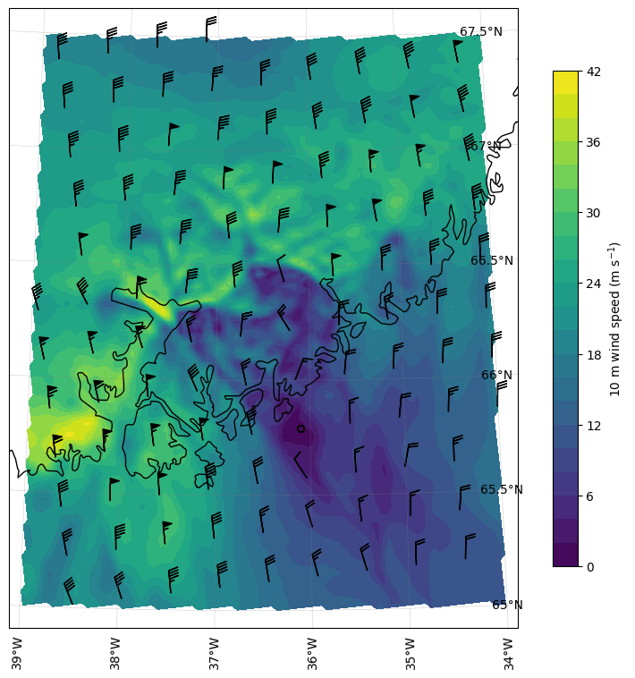
CARRA2: Retrieve and plot a sub-domain

In this notebook we demonstrate how to extract a sub-domain. Notice that the downloaded number of points using a sub-domain is the same as without, but anything outside the sub-domain is set to missing values, reducing the size of the data file significantly.

Load dependencies and create folders¶

In the first cell we load the relevant libraries for this notebook We also create folders for downloaded data and plots if we want to save them

import cartopy.crs as ccrs
import cartopy.feature as cfeature
import cdsapi
import cfgrib
import matplotlib.path as mpath
import matplotlib.pyplot as plt
import numpy as np
import os
import xarray as xr

Define your sub-domain¶

We first define the sub-domain as [N, W, S, E]. In our example, we choose the area around Tasiilaq, Greenland.

sub_domain = [67.5, -39, 65, -34]

Download fields¶

In the section below, fields are downloaded and stored. We will look at the wind speed at 2:00 AM UTC on Nov 15 2024. The resulting data file size is roughly 2Mb.

target_path = os.path.join('data', 'wind_speed_subdomain.grib')


dataset = "reanalysis-pan-carra"
request = {
    "level_type": "single_levels",
    "variable": [
        "10m_wind_direction",
        "10m_wind_speed"
    ],
    "product_type": "forecast",
    "time": ["00:00"],
    "leadtime_hour": ["2"],
    "year": ["2024"],
    "month": ["11"],
    "day": ["15"],
    "data_format": "grib",
    "area": sub_domain
}

client = cdsapi.Client()
client.retrieve(dataset, request).download(target_path)

ds = cfgrib.open_dataset(target_path)
ds

Plot the sub-domain¶

In this plot we now plot wind speed and direction

N, W, S, E = sub_domain
lat = ds.latitude
lon = ((ds.longitude + 180) % 360) - 180 

mask = (lat >= S) & (lat <= N) & (lon >= W) & (lon <= E)
ys, xs = np.where(mask.values)
sub = ds.isel(y=slice(ys.min(), ys.max() + 1),
              x=slice(xs.min(), xs.max() + 1))

sub_lat = sub.latitude
sub_lon = ((sub.longitude + 180) % 360) - 180

spd = sub["si10"]

# Converting to knots for plotting barbs
spd_kt = spd * 1.94384
wdir = np.deg2rad(sub["wdir10"])
u = -spd_kt * np.sin(wdir)
v = -spd_kt * np.cos(wdir)

step = max(1, min(sub.sizes["y"], sub.sizes["x"]) // 10)

proj = ccrs.NorthPolarStereo(central_longitude=-36.6)

fig = plt.figure(figsize=(10, 9))
ax = plt.axes(projection=proj)
ax.set_extent([W - .1, E + .1, S - .1, N + .1], crs=ccrs.PlateCarree())

mesh = ax.contourf(sub_lon, sub_lat, spd, levels=20,
                   transform=ccrs.PlateCarree(), cmap="viridis")
cbar = fig.colorbar(mesh, ax=ax, orientation="vertical", pad=0.05, shrink=0.8)
cbar.set_label("10 m wind speed (m s$^{-1}$)")

bx = sub_lon.values[::step, ::step].ravel()
by = sub_lat.values[::step, ::step].ravel()
bu = u.values[::step, ::step].ravel()
bv = v.values[::step, ::step].ravel()
valid = np.isfinite(bu) & np.isfinite(bv)
ax.barbs(bx[valid], by[valid], bu[valid], bv[valid],
         length=6, transform=ccrs.PlateCarree())

ax.coastlines(resolution="10m")
ax.add_feature(cfeature.BORDERS, linewidth=0.5)
gl = ax.gridlines(draw_labels=True, linewidth=0.3, color="gray", alpha=0.5)
gl.top_labels = False
gl.right_labels = False

fig.savefig(os.path.join("plots", "wind_speed_subdomain.png"),
            dpi=150, bbox_inches="tight")
plt.show()