Ocean regime prediction with Bayesian neural networks

Ocean regime prediction with Bayesian neural networks#

This notebook was last tested and operational on 16/06/2025. Please report any issues.

About

This notebook was originally created for ECMWF’s MOOC on Machine Learning in Weather and Climate, and has been lightly updated and tested for the purposes of this collection of examples. The original notebook can be found here.

The work in this notebook is based on Clare et al. (2022) Explainable Artificial Intelligence for Bayesian Neural Networks: Toward Trustworthy Predictions of Ocean Dynamics. This in turn builds on work in Sonnewald & Lguensat (2021) who built a deterministic neural network for the same problem and Sonnewald et al. (2019), where the ocean regimes were first identified by k-means clustering.

Running this notebook

This notebook can be run/accessed on the following free online platforms. Please note they are not officially supported by or linked with ECMWF. See Running the notebooks for more details.

Introduction#

In this notebook we will use a Bayesian neural network (BNN) to probabilistically classify ocean gridpoints into ocean circulation regimes.

A Bayesian neural network (BNN) is a type of neural network which treats the network parameters (weights and biases) as probability distributions rather than fixed estimates. As a result, predictions from a BNN a probabilistic (e.g. the probability of belonging to a particular class). BNNs are particularly useful for capturing uncertainty. They are typically trained by variational inference. See our ML MOOC (Tier 2, “Uncertainty and Generative Modelling module” for more details).

In this example we will use a set of input features (predictor variables) and the corresponding circulation regime labels, for each gridpoint, to train our model. We begin with a simple neural network, and add probabilistic features, to arrive at the full BNN. At the end of the notebook we also demonstrate how to analyse and visualise the uncertainty of the classifications from the BNN.

The input features for our neural network are as follows:

Wind stress curl
Mean Sea Surface Height (SSH) (20 years)
Gradients of Mean Sea Surface Height
Bathymetry
Gradients of bathymetry
Coriolis

For justification of this choice of these features please see Sonnewald & Lguensat (2021).

Set up your environment#

We’ll begin by loading the required packages. Importantly, tensorflow probability (which is what we will use to build the Bayesian neural networks) has an incompatibility with the latest version of keras. For this reason, we will have to install specific versions of tensorflow, tensorflow probability, and keras. Depending on which platform you run this notebook on (e.g. Colab), you may be told to restart your runtime - this may look like an error, but restart and carry on - it should work!

!pip install tensorflow==2.15.0
!pip install tensorflow-probability==0.23.0
!pip install keras==2.15.0

We’ll now load the libraries just installed, and check the versions.

import tensorflow as tf
import tensorflow_probability as tfp
import tf_keras as keras  # Make sure tf-keras==2.15.0 is installed

print("TensorFlow version:", tf.__version__)
print("TFP version:", tfp.__version__)
print("Keras version:", keras.__version__)
print("Keras package location:", keras.__file__)

TensorFlow version: 2.15.0
TFP version: 0.23.0
Keras version: 2.18.0
Keras package location: /usr/local/lib/python3.11/dist-packages/tf_keras/__init__.py

Finally, we will import the standard libraries for working with array data, and plotting.

# 📊 Standard packages for data and plotting
import numpy as np
import xarray as xr
from scipy.io import loadmat
import matplotlib.pyplot as plt

Download data#

We now download the data, which is hosted on an ECMWF server. The following commands download:

Labels for ocean circulation regimes
Wind stress curl
Sea surface height for years 1992-2011
Bathymetry data

Some of these variables will be used directly as predictors, while further predictors will be created by operating on them. Notice that the files we download are in a mixture of file formats. This may take a few minutes to complete.

## Download input Data
! wget https://get.ecmwf.int/repository/mooc-machine-learning-weather-climate/tier_2/uncertainty/kCluster6.npy
! wget https://get.ecmwf.int/repository/mooc-machine-learning-weather-climate/tier_2/uncertainty/curlTau.npy
! wget https://get.ecmwf.int/repository/mooc-machine-learning-weather-climate/tier_2/uncertainty/SSHdata/SSH.1992.nc
! wget https://get.ecmwf.int/repository/mooc-machine-learning-weather-climate/tier_2/uncertainty/SSHdata/SSH.1993.nc
! wget https://get.ecmwf.int/repository/mooc-machine-learning-weather-climate/tier_2/uncertainty/SSHdata/SSH.1994.nc
! wget https://get.ecmwf.int/repository/mooc-machine-learning-weather-climate/tier_2/uncertainty/SSHdata/SSH.1995.nc
! wget https://get.ecmwf.int/repository/mooc-machine-learning-weather-climate/tier_2/uncertainty/SSHdata/SSH.1996.nc
! wget https://get.ecmwf.int/repository/mooc-machine-learning-weather-climate/tier_2/uncertainty/SSHdata/SSH.1997.nc
! wget https://get.ecmwf.int/repository/mooc-machine-learning-weather-climate/tier_2/uncertainty/SSHdata/SSH.1998.nc
! wget https://get.ecmwf.int/repository/mooc-machine-learning-weather-climate/tier_2/uncertainty/SSHdata/SSH.1999.nc
! wget https://get.ecmwf.int/repository/mooc-machine-learning-weather-climate/tier_2/uncertainty/SSHdata/SSH.2000.nc
! wget https://get.ecmwf.int/repository/mooc-machine-learning-weather-climate/tier_2/uncertainty/SSHdata/SSH.2001.nc
! wget https://get.ecmwf.int/repository/mooc-machine-learning-weather-climate/tier_2/uncertainty/SSHdata/SSH.2002.nc
! wget https://get.ecmwf.int/repository/mooc-machine-learning-weather-climate/tier_2/uncertainty/SSHdata/SSH.2003.nc
! wget https://get.ecmwf.int/repository/mooc-machine-learning-weather-climate/tier_2/uncertainty/SSHdata/SSH.2004.nc
! wget https://get.ecmwf.int/repository/mooc-machine-learning-weather-climate/tier_2/uncertainty/SSHdata/SSH.2005.nc
! wget https://get.ecmwf.int/repository/mooc-machine-learning-weather-climate/tier_2/uncertainty/SSHdata/SSH.2006.nc
! wget https://get.ecmwf.int/repository/mooc-machine-learning-weather-climate/tier_2/uncertainty/SSHdata/SSH.2007.nc
! wget https://get.ecmwf.int/repository/mooc-machine-learning-weather-climate/tier_2/uncertainty/SSHdata/SSH.2008.nc
! wget https://get.ecmwf.int/repository/mooc-machine-learning-weather-climate/tier_2/uncertainty/SSHdata/SSH.2009.nc
! wget https://get.ecmwf.int/repository/mooc-machine-learning-weather-climate/tier_2/uncertainty/SSHdata/SSH.2010.nc
! wget https://get.ecmwf.int/repository/mooc-machine-learning-weather-climate/tier_2/uncertainty/SSHdata/SSH.2011.nc
! wget https://get.ecmwf.int/repository/mooc-machine-learning-weather-climate/tier_2/uncertainty/H_wHFacC.mat

Create predictor and target variables#

Currently, our data is inside downloaded files. We need to import it into Python, and apply some processing operations to create our cleaned data set ready for training and modelling.

We’ll begin with our target variable - the ocean regimes labels. This simply requires importing the .npy file and replacing land pixels with NaNs.

## Load in ocean regimes labels as target data. These ocean regimes were determined in Sonnewald et al. 2019
ecco_label = np.transpose(np.load('kCluster6.npy'))

# replace land pixels by NaNs
ecco_label[ecco_label==-1] = np.nan

We now move to the predictor variables. Two of our variables can be generated directly: wind stress curl by importing the data from a .npy (NumPy array) file, and bathymetry data from a MATLAB file.

wind_stress_curl = np.transpose(np.load('curlTau.npy'))
bathymetry = np.transpose(loadmat('H_wHFacC.mat')['val'])

The next predictor variable, mean sea surface height (SSH), is created by reading in all SSH.* files (which are NetCDF files), combining by coordinates (using xarray), and then taking the mean at each coordinate.

monthly_ssh = xr.open_mfdataset('SSH.*.nc', combine='by_coords')
SSH20mean = monthly_ssh['SSH'].mean(axis=0).values  # 20 years mean of sea surface height

Next we’ll calculate the Coriolis parameter using the latitude values in the monthly SSH variable created previously. This is also included as a predictor variable.

# get latitudes
lat = monthly_ssh['lat'].values

##coriolis
Omega=7.2921e-5 # coriolis parameter
f = (2*Omega*np.sin(lat*np.pi/180))

Finally, we’ll create the gradients of SSH and bathymetry in the latitude and longitude directions. These gradients highlight spatial changes, which are relevant for understanding ocean circulation patterns.

## Calculate the SSH gradients, bathymetry gradients and coriolis

lonRoll = np.roll(monthly_ssh['lat'].values, axis=0, shift=-1)
Londiff = lonRoll - monthly_ssh['lat'].values  # equivalent to doing x_{i} - x_{i-1}

latDiff=1.111774765625000e+05
latY=np.gradient(lat, axis=0)*latDiff
lonX=np.abs(np.cos(lat*np.pi/180))*latDiff*Londiff

def grad(d,y,x):
    grady=np.gradient(d, axis=0)/y
    gradx=np.gradient(d, axis=1)/x
    return grady, gradx

gradSSH_y, gradSSH_x = grad(SSH20mean,latY,lonX)
gradBathm_y, gradBathm_x = grad(bathymetry,latY,lonX)

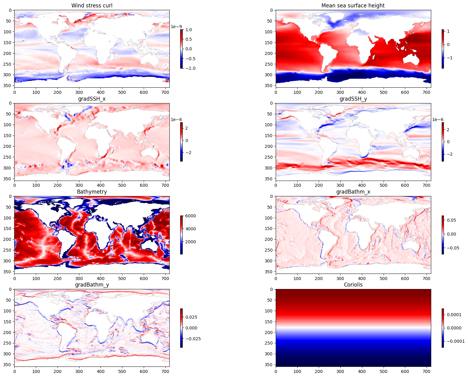
Plot data#

We now have a unified data set. Before training our models, we will plot the predictor variables that we created in the previous section on a map. This is simply to visualise the spatial patterns of our data.

## Plot data

plt.figure(figsize=(20,15))

plt.subplot(4,2,1)
plt.imshow(np.flipud(wind_stress_curl), cmap='seismic')
plt.colorbar(shrink=0.5)
plt.clim(-1e-9,1e-9)
plt.title('Wind stress curl')

plt.subplot(4,2,2)
plt.imshow(np.flipud(SSH20mean), cmap='seismic')
plt.colorbar(shrink=0.5)
plt.title('Mean sea surface height')

plt.subplot(4,2,3)
plt.imshow(np.flipud(gradSSH_x), cmap='seismic')
plt.colorbar(shrink=0.5)
plt.title('gradSSH_x')

plt.subplot(4,2,4)
plt.imshow(np.flipud(gradSSH_y), cmap='seismic')
plt.colorbar(shrink=0.5)
plt.title('gradSSH_y')

plt.subplot(4,2,5)
plt.imshow(np.flipud(bathymetry), cmap='seismic')
plt.colorbar(shrink=0.5)
plt.title('Bathymetry')

plt.subplot(4,2,6)
plt.imshow(np.flipud(gradBathm_x), cmap='seismic')
plt.colorbar(shrink=0.5)
plt.title('gradBathm_x')

plt.subplot(4,2,7)
plt.imshow(np.flipud(gradBathm_y), cmap='seismic')
plt.colorbar(shrink=0.5)
plt.title('gradBathm_y')

plt.subplot(4,2,8)
plt.imshow(np.flipud(f), cmap='seismic')
plt.colorbar(shrink=0.5)
plt.title('Coriolis')

plt.show()

_images/ad142e6982e2e03b2a7b44624b3029852669333de5419e06cfe02243a52d2a63.png

Create training and test sets#

In this section we will prepare the data set for the model - by creating training and testing sets and standardising the data. In the following code cell we will do two things:

Flag any points that have missing (NaN) values in any of the predictor variables. These will be excluded from the data set.
Create masks to define training and test datasets. The training set will include all ocean points except (roughly) the Atlantic Ocean. The test set is the inverse, including only the Atlantic Ocean.

## Mask land pixels and other noisy locations
missingdataindex = np.isnan(wind_stress_curl*SSH20mean*gradSSH_x*gradSSH_y*bathymetry*gradBathm_x*gradBathm_y)

## Training data is ocean dataset excluding the Atlantic Ocean
maskTraining = (~missingdataindex).copy()
maskTraining[:,200:400]=False

## Test dataset is Atlantic Ocean dataset
maskTest = (~missingdataindex).copy()
maskTest[:,list(range(200))+list(range(400,720))]=False

We now use these masks to compile the full, training and test datasets. The output of this cell also gives the dimensions of the resulting arrays.

## Set up training and test datasets

TotalDataset = np.stack((wind_stress_curl[~missingdataindex],
                         SSH20mean[~missingdataindex],
                         gradSSH_x[~missingdataindex],
                         gradSSH_y[~missingdataindex],
                         bathymetry[~missingdataindex],
                         gradBathm_x[~missingdataindex],
                         gradBathm_y[~missingdataindex],
                         f[~missingdataindex]),1)

TrainDataset = np.stack((wind_stress_curl[maskTraining],
                         SSH20mean[maskTraining],
                         gradSSH_x[maskTraining],
                         gradSSH_y[maskTraining],
                         bathymetry[maskTraining],
                         gradBathm_x[maskTraining],
                         gradBathm_y[maskTraining],
                         f[maskTraining]),1)

TestDataset = np.stack((wind_stress_curl[maskTest],
                         SSH20mean[maskTest],
                         gradSSH_x[maskTest],
                         gradSSH_y[maskTest],
                         bathymetry[maskTest],
                         gradBathm_x[maskTest],
                         gradBathm_y[maskTest],
                       f[maskTest]),1)

print(TotalDataset.shape, TrainDataset.shape, TestDataset.shape)

train_label = ecco_label[maskTraining]
test_label = ecco_label[maskTest]
print(train_label.shape, test_label.shape)

(149587, 8) (109259, 8) (40328, 8)
(109259,) (40328,)

The final step here is to standardise the data so that each variable has mean zero and unit variance. This ensures that variables are on a similar scale, and improves the model performance and stability.

## Scale the data

from sklearn.preprocessing import StandardScaler
scaler = StandardScaler()
scaler.fit(TrainDataset)
scaler.mean_,scaler.scale_

X_train_scaled = scaler.transform(TrainDataset)
X_test_scaled = scaler.transform(TestDataset)

Our data is finally ready for modelling. To build the Bayesian Neural Network (BNN) we’ll be using both tensorflow and tensorflow_probability (imported previously). We will also convert the target labels into a one-hot encoded format which is suitable for tensorflow.

# aliases for some modules
tfd = tfp.distributions
tfpl = tfp.layers

# convert target labels to appropriate data type for tensorflow
Y_train = tf.keras.utils.to_categorical(train_label)
Y_test = tf.keras.utils.to_categorical(test_label)

Deterministic model#

To begin with we will build a standard feedforward neural network where the parameters are fixed values, i.e. a deterministic model. Our model takes the eight predictor variables as inputs, and processes it through several hidden layers. The final layer uses a softmax function to classify the result into one of the six ocean circulation regimes.

The data is shaped for a gridpoint-by-gridpoint approach so dense layers are appropriate here. The following function defines the model using a sequential approach, and it is fitted to the training data in the next step.

from keras.models import Sequential, Model
from keras.layers import Input, Dense
from keras.optimizers import RMSprop

def deterministic_model():
    model = Sequential([
      Dense(input_shape = (8,), units =24,
                            activation = tf.keras.activations.tanh),
      Dense(units =24, activation = tf.keras.activations.tanh),
      Dense(units =16, activation = tf.keras.activations.tanh),
      Dense(units =16, activation = tf.keras.activations.tanh),
      Dense(units =6, activation = tf.keras.activations.softmax),
      ])
    return model

It’s now time to train the model on the training data. We have to configure how the model will be trained. We specify:

The categorical cross-entropy loss function, which quantifies the difference between the model class predictions and the true labels.
The categorical accuracy metric is simply a metric which is reported during training to help monitor and evaluate the model performance.
The optimiser is specified as the Adam optimiser, with learning rate 0.01.

We also specify how the model will be trained:

Batch size of 32
Number of epochs is 10

The batch size, number of epochs, optimiser type and configuration can all affect the performance of the model and are considered hyperparameters. We could potentially adjust these to see if model performance could be improved, but we leave that as an exercise for the reader.

# Compile and fit the deterministic model
det_model = deterministic_model()
det_model.summary()
det_model.compile(loss = 'categorical_crossentropy', metrics = ['categorical_accuracy'],
              optimizer=tf.keras.optimizers.Adam(learning_rate=0.01))
det_model.fit(X_train_scaled, Y_train,
                    batch_size=32,
                    epochs=10,
                    verbose=1,
                    validation_split = 0.2, shuffle = True)

Model: "sequential"
_________________________________________________________________
 Layer (type)                Output Shape              Param #   
=================================================================
 dense (Dense)               (None, 24)                216       
                                                                 
 dense_1 (Dense)             (None, 24)                600       
                                                                 
 dense_2 (Dense)             (None, 16)                400       
                                                                 
 dense_3 (Dense)             (None, 16)                272       
                                                                 
 dense_4 (Dense)             (None, 6)                 102       
                                                                 
=================================================================
Total params: 1590 (6.21 KB)
Trainable params: 1590 (6.21 KB)
Non-trainable params: 0 (0.00 Byte)
_________________________________________________________________
Epoch 1/10
2732/2732 [==============================] - 12s 4ms/step - loss: 0.3932 - categorical_accuracy: 0.8552 - val_loss: 0.7386 - val_categorical_accuracy: 0.7276
Epoch 2/10
2732/2732 [==============================] - 10s 4ms/step - loss: 0.3190 - categorical_accuracy: 0.8831 - val_loss: 0.6685 - val_categorical_accuracy: 0.8390
Epoch 3/10
2732/2732 [==============================] - 8s 3ms/step - loss: 0.3075 - categorical_accuracy: 0.8864 - val_loss: 0.6583 - val_categorical_accuracy: 0.8306
Epoch 4/10
2732/2732 [==============================] - 6s 2ms/step - loss: 0.3016 - categorical_accuracy: 0.8878 - val_loss: 0.7168 - val_categorical_accuracy: 0.7928
Epoch 5/10
2732/2732 [==============================] - 6s 2ms/step - loss: 0.2948 - categorical_accuracy: 0.8898 - val_loss: 0.7298 - val_categorical_accuracy: 0.7852
Epoch 6/10
2732/2732 [==============================] - 7s 2ms/step - loss: 0.2954 - categorical_accuracy: 0.8895 - val_loss: 0.6632 - val_categorical_accuracy: 0.8083
Epoch 7/10
2732/2732 [==============================] - 5s 2ms/step - loss: 0.2921 - categorical_accuracy: 0.8901 - val_loss: 0.6299 - val_categorical_accuracy: 0.8056
Epoch 8/10
2732/2732 [==============================] - 7s 2ms/step - loss: 0.2931 - categorical_accuracy: 0.8908 - val_loss: 0.6076 - val_categorical_accuracy: 0.7886
Epoch 9/10
2732/2732 [==============================] - 6s 2ms/step - loss: 0.2925 - categorical_accuracy: 0.8926 - val_loss: 0.6119 - val_categorical_accuracy: 0.8052
Epoch 10/10
2732/2732 [==============================] - 6s 2ms/step - loss: 0.2908 - categorical_accuracy: 0.8905 - val_loss: 0.6295 - val_categorical_accuracy: 0.8119

<keras.src.callbacks.History at 0x785b29d334d0>

Having fitted the model, we check its accuracy. We feed both the training and test data into the model.

# Evaluate the accuracy of this deterministic model

print(det_model.evaluate(X_train_scaled, Y_train))
print(det_model.evaluate(X_test_scaled, Y_test))

3415/3415 [==============================] - 5s 1ms/step - loss: 0.3486 - categorical_accuracy: 0.8832
[0.3486475646495819, 0.8832132816314697]
1261/1261 [==============================] - 2s 1ms/step - loss: 0.5557 - categorical_accuracy: 0.7981
[0.5557481646537781, 0.7981055378913879]

The main metric of interest here is the performance on the test set. This shows a categorical accuracy of about 77-80% (this will vary each time the model is trained, due to the randomness built in to the training process, e.g. sampling).

Probabilistic model#

In this section we will extend our model so that it provides a probabilistic output rather than deterministic categories, quantifying the aleatoric uncertainty. In the model specification this simply means replacing the softmax output layer from the previous model with a “OneHotCategorical” Layer from Tensorflow probability. As a result, the output of the network is a distribution rather than a categorical value. However, the weights and biases are still fixed parameters, so the model is not yet fully Bayesian (we build the full Bayesian model in the next section).

def probabilistic_model():
    inputs = Input(shape=(8,))
    x = Dense(units=24, activation=tf.keras.activations.tanh)(inputs)
    x = Dense(units=24, activation=tf.keras.activations.tanh)(x)
    x = Dense(units=16, activation=tf.keras.activations.tanh)(x)
    x = Dense(units=16, activation=tf.keras.activations.tanh)(x)
    logits = Dense(units=6, activation=None)(x)
    outputs = tfpl.OneHotCategorical(6)(logits)

    model = Model(inputs=inputs, outputs=outputs)
    return model

prob_model = probabilistic_model()
prob_model.summary()

Model: "model"
_________________________________________________________________
 Layer (type)                Output Shape              Param #   
=================================================================
 input_1 (InputLayer)        [(None, 8)]               0         
                                                                 
 dense_5 (Dense)             (None, 24)                216       
                                                                 
 dense_6 (Dense)             (None, 24)                600       
                                                                 
 dense_7 (Dense)             (None, 16)                400       
                                                                 
 dense_8 (Dense)             (None, 16)                272       
                                                                 
 dense_9 (Dense)             (None, 6)                 102       
                                                                 
 one_hot_categorical (OneHo  ((None, 6),               0         
 tCategorical)                (None, 6))                         
                                                                 
=================================================================
Total params: 1590 (6.21 KB)
Trainable params: 1590 (6.21 KB)
Non-trainable params: 0 (0.00 Byte)
_________________________________________________________________

We now fit the model to the training data as we did in the last example. A difference here though is that we have to define a new loss function which calculates the loss between the probabilistic output of the model and the true labels. Our loss function is the negative log-likelihood function, which calculates the log probability of the true labels under the predicted distribution y_pred.log_prob(y_true) and then negates it to get the negative log-likelihood.

In other respects, the configuration of the model training is similar to before.

# define the negative log-likelihood function
def nll(y_true, y_pred):
    return -y_pred.log_prob(y_true)

prob_model.compile(loss=nll,
              optimizer=tf.keras.optimizers.Adam(learning_rate=0.01),
              metrics=['accuracy'])

prob_model.fit(X_train_scaled, Y_train,
                    batch_size=32,
                    epochs=20,
                    verbose=1,
                    validation_split = 0.2, shuffle = True)

Epoch 1/20
2732/2732 [==============================] - 8s 2ms/step - loss: 0.3893 - accuracy: 0.7915 - val_loss: 0.7627 - val_accuracy: 0.7069
Epoch 2/20
2732/2732 [==============================] - 6s 2ms/step - loss: 0.3175 - accuracy: 0.8330 - val_loss: 0.5796 - val_accuracy: 0.7345
Epoch 3/20
2732/2732 [==============================] - 10s 4ms/step - loss: 0.3069 - accuracy: 0.8387 - val_loss: 0.6163 - val_accuracy: 0.7351
Epoch 4/20
2732/2732 [==============================] - 7s 3ms/step - loss: 0.3027 - accuracy: 0.8394 - val_loss: 0.5682 - val_accuracy: 0.7595
Epoch 5/20
2732/2732 [==============================] - 6s 2ms/step - loss: 0.2972 - accuracy: 0.8429 - val_loss: 0.6595 - val_accuracy: 0.7368
Epoch 6/20
2732/2732 [==============================] - 6s 2ms/step - loss: 0.2895 - accuracy: 0.8476 - val_loss: 0.5717 - val_accuracy: 0.7805
Epoch 7/20
2732/2732 [==============================] - 6s 2ms/step - loss: 0.2890 - accuracy: 0.8461 - val_loss: 0.5995 - val_accuracy: 0.7644
Epoch 8/20
2732/2732 [==============================] - 6s 2ms/step - loss: 0.2862 - accuracy: 0.8489 - val_loss: 0.7279 - val_accuracy: 0.7406
Epoch 9/20
2732/2732 [==============================] - 6s 2ms/step - loss: 0.2941 - accuracy: 0.8449 - val_loss: 0.6622 - val_accuracy: 0.7391
Epoch 10/20
2732/2732 [==============================] - 6s 2ms/step - loss: 0.2969 - accuracy: 0.8428 - val_loss: 0.7861 - val_accuracy: 0.7430
Epoch 11/20
2732/2732 [==============================] - 7s 2ms/step - loss: 0.2913 - accuracy: 0.8459 - val_loss: 0.6307 - val_accuracy: 0.7557
Epoch 12/20
2732/2732 [==============================] - 5s 2ms/step - loss: 0.2879 - accuracy: 0.8487 - val_loss: 0.6138 - val_accuracy: 0.7694
Epoch 13/20
2732/2732 [==============================] - 6s 2ms/step - loss: 0.2961 - accuracy: 0.8436 - val_loss: 0.5991 - val_accuracy: 0.7944
Epoch 14/20
2732/2732 [==============================] - 6s 2ms/step - loss: 0.2970 - accuracy: 0.8437 - val_loss: 0.6161 - val_accuracy: 0.7577
Epoch 15/20
2732/2732 [==============================] - 7s 3ms/step - loss: 0.2981 - accuracy: 0.8435 - val_loss: 0.6826 - val_accuracy: 0.7522
Epoch 16/20
2732/2732 [==============================] - 6s 2ms/step - loss: 0.2864 - accuracy: 0.8479 - val_loss: 0.6687 - val_accuracy: 0.7680
Epoch 17/20
2732/2732 [==============================] - 6s 2ms/step - loss: 0.2933 - accuracy: 0.8457 - val_loss: 0.6750 - val_accuracy: 0.7622
Epoch 18/20
2732/2732 [==============================] - 6s 2ms/step - loss: 0.2883 - accuracy: 0.8489 - val_loss: 0.6707 - val_accuracy: 0.7480
Epoch 19/20
2732/2732 [==============================] - 7s 2ms/step - loss: 0.2938 - accuracy: 0.8422 - val_loss: 0.6140 - val_accuracy: 0.7720
Epoch 20/20
2732/2732 [==============================] - 6s 2ms/step - loss: 0.3026 - accuracy: 0.8418 - val_loss: 0.6702 - val_accuracy: 0.7811

<keras.src.callbacks.History at 0x785b15d620d0>

An example of the output of this trained model is given below. Each value in the array gives the estimated probability of the input data point belonging to each of the six ocean circulation regimes.

## Example output
prob_model(X_test_scaled[0:1]).mean().numpy()

array([[2.23020121e-04, 6.34492701e-03, 6.81366203e-07, 2.56378025e-01,
        1.03569975e-04, 7.36949801e-01]], dtype=float32)

As before, we will evaluate the accuracy of the model.

# Evaluate the accuracy of this first Bayesian model

print(prob_model.evaluate(X_train_scaled, Y_train))
print(prob_model.evaluate(X_test_scaled, Y_test))

3415/3415 [==============================] - 5s 1ms/step - loss: 0.3630 - accuracy: 0.8366
[0.3630378544330597, 0.8365535140037537]
1261/1261 [==============================] - 2s 1ms/step - loss: 0.5692 - accuracy: 0.7627
[0.5691739320755005, 0.7626959085464478]

Probabilistic model (epistemic)#

In this section we will further extend our model to quantify epistemic uncertainty as well as aleatoric uncertainty. This means that the weights and biases of the model will now be treated as random variables, rather than fixed parameters. Building a Bayesian model requires defining prior distributions of these trainable parameters.

Our goal is to find the posterior distributions of these parameters, and this will be done with variational inference, which is a technique in Bayesian statistics used to approximate complex probability distributions, especially when exact inference is computationally intractable. Varational inference requires additionally specifying a distribution type for the posterior, so we have to define this as well.

The following function specifies the prior distribution for the weights and biases in one of the layers of our model. It uses a multivariate normal distribution with mean zero and standard deviation 1. This assumes that parameters are independent.

# Define the prior weight distribution -- all N(0, 1) -- and not trainable
def prior(kernel_size, bias_size, dtype = None):
    n = kernel_size + bias_size
    prior_model = Sequential([
                            tfpl.DistributionLambda(
                                lambda t: tfd.MultivariateNormalDiag(loc = tf.zeros(n), scale_diag = tf.ones(n))
                            )
    ]) # normal distribution for each weight in the layer
    return prior_model

This next function defines the type of the posterior distribution of the parameters in a layer, for the purposes of variational inference. The posterior is assumed to be shaped as a multivariate normal distribution - the task will be to learn the parameters of this distribution (means and variances).

# Define variational posterior weight distribution -- multivariate Gaussian
def posterior(kernel_size, bias_size, dtype = None):
    n = kernel_size + bias_size
    posterior_model = Sequential([
                tfpl.VariableLayer(2*n, dtype=dtype),
                tfpl.DistributionLambda (
        lambda t: tfd.MultivariateNormalDiag(loc = t[..., :n], scale_diag = tf.math.exp(t[..., n:])))
    ]) # define posterior for each weight in the layer
    return posterior_model

Now we can define the model. The Dense layers used in the previous models are replaced with DenseVariational layers from tensorflow_probability. In each layer, we specify the prior and posterior distributions using the functions defined previously. The shape of the model is however similar to the previous models: the hidden layers have 24, 24, 16, and 16 units, while the final layer has 6 units, corresponding to the number of ocean circulation regimes.

There is a technical issue here: variational inference uses the Kullback-Leibler divergence to quantify the difference between the approximate posterior and the prior, encouraging the model’s learned parameters to stay relatively close to the prior values. We have to scale the KL distance by the reciprocal of the number of training samples to ensure it is balanced with the negative log-likelihood. This is specified in the kl_weight argument.

def bnn():
  model = Sequential([
    tfpl.DenseVariational(input_shape = (8,), units =24,
                          activation = tf.keras.activations.tanh,
                          make_prior_fn=prior,
                          make_posterior_fn=posterior,
                          kl_weight = 1/X_train_scaled.shape[0], # have to rescale the kl_error
                          kl_use_exact=True # use if have analytic form of prior and posterior - may error in which case change to False
                          ),
    tfpl.DenseVariational(units =24,
                          activation = tf.keras.activations.tanh,
                          make_prior_fn=prior,
                          make_posterior_fn=posterior,
                          kl_weight = 1/X_train_scaled.shape[0], # have to rescale the kl_error
                          kl_use_exact=True # use if have analytic form of prior and posterior - may error in which case change to False
                          ),
    tfpl.DenseVariational(units =16,
                          activation = tf.keras.activations.tanh,
                          make_prior_fn=prior,
                          make_posterior_fn=posterior,
                          kl_weight = 1/X_train_scaled.shape[0], # have to rescale the kl_error
                          kl_use_exact=True # use if have analytic form of prior and posterior - may error in which case change to False
                          ),
    tfpl.DenseVariational(units =16,
                          activation = tf.keras.activations.tanh,
                          make_prior_fn=prior,
                          make_posterior_fn=posterior,
                          kl_weight = 1/X_train_scaled.shape[0], # have to rescale the kl_error
                          kl_use_exact=True # use if have analytic form of prior and posterior - may error in which case change to False
                          ),
    tfpl.DenseVariational(units =6,
                          make_prior_fn=prior,
                          make_posterior_fn=posterior,
                          kl_weight = 1/X_train_scaled.shape[0], # have to rescale the kl_error
                          kl_use_exact=True # use if have analytic form of prior and posterior - may error in which case change to False
                          ),
   tfpl.OneHotCategorical(6)])
  return model

Next we will specify how the model should be trained:

We use the negative log-likelihood function as the loss function.
We compile the model, specifying the optimiser and learning rate.
We add “callbacks”, which are functions executed at specific stages of the training process. In this case, checkpoint_callback saves the model weights after each epoch, and reduce_lr_callback adjusts the learning rate based on the validation loss, in order to improve convergence.

bnn_model = bnn()

# negative log-likelihood as loss function
def nll(y_true, y_pred):
    return -y_pred.log_prob(y_true)

bnn_model.compile(loss=nll,
              optimizer=tf.keras.optimizers.Adam(learning_rate=0.01),
              metrics=['accuracy'])

# add callbacks to save best weights
checkpoint_callback = tf.keras.callbacks.ModelCheckpoint(
    'bnn_weights.h5', monitor='val_loss', verbose=1, save_best_only=True,
    save_weights_only=True, mode='auto', save_freq='epoch')

# and to reduce the learning rate if the error does not improve after 15 epochs
reduce_lr_callback = tf.keras.callbacks.ReduceLROnPlateau(
            monitor = 'val_loss',
            patience=15,
            factor=0.25,
            verbose=1)

Finally we can train the model. Here we will use a maximum of 100 epochs due to the increased complexity of the model, so this may take some time to train.

# fit model
bnn_model.fit(X_train_scaled, Y_train,
                    batch_size=32,
                    epochs=100,
                    verbose=1,
                    validation_split = 0.2, shuffle = True,
                    callbacks = [checkpoint_callback, reduce_lr_callback])

Epoch 1/100
2716/2732 [============================>.] - ETA: 0s - loss: 2.0595 - accuracy: 0.2086
Epoch 1: val_loss improved from inf to 1.65217, saving model to bnn_weights.h5
2732/2732 [==============================] - 14s 3ms/step - loss: 2.0575 - accuracy: 0.2087 - val_loss: 1.6522 - val_accuracy: 0.2247 - lr: 0.0100
Epoch 2/100
2719/2732 [============================>.] - ETA: 0s - loss: 1.6896 - accuracy: 0.2134
Epoch 2: val_loss improved from 1.65217 to 1.61870, saving model to bnn_weights.h5
2732/2732 [==============================] - 7s 2ms/step - loss: 1.6896 - accuracy: 0.2135 - val_loss: 1.6187 - val_accuracy: 0.2280 - lr: 0.0100
Epoch 3/100
2725/2732 [============================>.] - ETA: 0s - loss: 1.2785 - accuracy: 0.3472
Epoch 3: val_loss improved from 1.61870 to 1.56400, saving model to bnn_weights.h5
2732/2732 [==============================] - 8s 3ms/step - loss: 1.2775 - accuracy: 0.3475 - val_loss: 1.5640 - val_accuracy: 0.3342 - lr: 0.0100
Epoch 4/100
2718/2732 [============================>.] - ETA: 0s - loss: 0.8105 - accuracy: 0.5727
Epoch 4: val_loss improved from 1.56400 to 1.27257, saving model to bnn_weights.h5
2732/2732 [==============================] - 8s 3ms/step - loss: 0.8099 - accuracy: 0.5730 - val_loss: 1.2726 - val_accuracy: 0.4965 - lr: 0.0100
Epoch 5/100
2720/2732 [============================>.] - ETA: 0s - loss: 0.6675 - accuracy: 0.6482
Epoch 5: val_loss improved from 1.27257 to 0.98727, saving model to bnn_weights.h5
2732/2732 [==============================] - 7s 2ms/step - loss: 0.6674 - accuracy: 0.6482 - val_loss: 0.9873 - val_accuracy: 0.6188 - lr: 0.0100
Epoch 6/100
2731/2732 [============================>.] - ETA: 0s - loss: 0.5797 - accuracy: 0.7105
Epoch 6: val_loss did not improve from 0.98727
2732/2732 [==============================] - 7s 3ms/step - loss: 0.5797 - accuracy: 0.7106 - val_loss: 0.9895 - val_accuracy: 0.6151 - lr: 0.0100
Epoch 7/100
2729/2732 [============================>.] - ETA: 0s - loss: 0.5493 - accuracy: 0.7296
Epoch 7: val_loss did not improve from 0.98727
2732/2732 [==============================] - 7s 2ms/step - loss: 0.5492 - accuracy: 0.7297 - val_loss: 1.0019 - val_accuracy: 0.5913 - lr: 0.0100
Epoch 8/100
2719/2732 [============================>.] - ETA: 0s - loss: 0.5350 - accuracy: 0.7398
Epoch 8: val_loss did not improve from 0.98727
2732/2732 [==============================] - 8s 3ms/step - loss: 0.5353 - accuracy: 0.7396 - val_loss: 0.9963 - val_accuracy: 0.6072 - lr: 0.0100
Epoch 9/100
2720/2732 [============================>.] - ETA: 0s - loss: 0.5231 - accuracy: 0.7402
Epoch 9: val_loss improved from 0.98727 to 0.97494, saving model to bnn_weights.h5
2732/2732 [==============================] - 11s 4ms/step - loss: 0.5234 - accuracy: 0.7400 - val_loss: 0.9749 - val_accuracy: 0.6251 - lr: 0.0100
Epoch 10/100
2725/2732 [============================>.] - ETA: 0s - loss: 0.5359 - accuracy: 0.7370
Epoch 10: val_loss improved from 0.97494 to 0.95721, saving model to bnn_weights.h5
2732/2732 [==============================] - 12s 4ms/step - loss: 0.5356 - accuracy: 0.7371 - val_loss: 0.9572 - val_accuracy: 0.6544 - lr: 0.0100
Epoch 11/100
2725/2732 [============================>.] - ETA: 0s - loss: 0.5233 - accuracy: 0.7482
Epoch 11: val_loss improved from 0.95721 to 0.89757, saving model to bnn_weights.h5
2732/2732 [==============================] - 7s 3ms/step - loss: 0.5234 - accuracy: 0.7482 - val_loss: 0.8976 - val_accuracy: 0.6760 - lr: 0.0100
Epoch 12/100
2719/2732 [============================>.] - ETA: 0s - loss: 0.4971 - accuracy: 0.7628
Epoch 12: val_loss did not improve from 0.89757
2732/2732 [==============================] - 7s 3ms/step - loss: 0.4973 - accuracy: 0.7628 - val_loss: 1.1582 - val_accuracy: 0.6074 - lr: 0.0100
Epoch 13/100
2725/2732 [============================>.] - ETA: 0s - loss: 0.5032 - accuracy: 0.7575
Epoch 13: val_loss did not improve from 0.89757
2732/2732 [==============================] - 7s 2ms/step - loss: 0.5033 - accuracy: 0.7575 - val_loss: 1.1306 - val_accuracy: 0.5954 - lr: 0.0100
Epoch 14/100
2730/2732 [============================>.] - ETA: 0s - loss: 0.4939 - accuracy: 0.7659
Epoch 14: val_loss did not improve from 0.89757
2732/2732 [==============================] - 10s 4ms/step - loss: 0.4939 - accuracy: 0.7659 - val_loss: 0.9871 - val_accuracy: 0.6556 - lr: 0.0100
Epoch 15/100
2709/2732 [============================>.] - ETA: 0s - loss: 0.4832 - accuracy: 0.7744
Epoch 15: val_loss did not improve from 0.89757
2732/2732 [==============================] - 9s 3ms/step - loss: 0.4834 - accuracy: 0.7741 - val_loss: 1.1157 - val_accuracy: 0.5817 - lr: 0.0100
Epoch 16/100
2712/2732 [============================>.] - ETA: 0s - loss: 0.4997 - accuracy: 0.7645
Epoch 16: val_loss did not improve from 0.89757
2732/2732 [==============================] - 7s 2ms/step - loss: 0.4997 - accuracy: 0.7645 - val_loss: 1.0366 - val_accuracy: 0.6333 - lr: 0.0100
Epoch 17/100
2722/2732 [============================>.] - ETA: 0s - loss: 0.4807 - accuracy: 0.7742
Epoch 17: val_loss did not improve from 0.89757
2732/2732 [==============================] - 7s 3ms/step - loss: 0.4808 - accuracy: 0.7740 - val_loss: 1.0578 - val_accuracy: 0.6425 - lr: 0.0100
Epoch 18/100
2719/2732 [============================>.] - ETA: 0s - loss: 0.4898 - accuracy: 0.7621
Epoch 18: val_loss did not improve from 0.89757
2732/2732 [==============================] - 8s 3ms/step - loss: 0.4899 - accuracy: 0.7619 - val_loss: 1.2762 - val_accuracy: 0.5897 - lr: 0.0100
Epoch 19/100
2715/2732 [============================>.] - ETA: 0s - loss: 0.4914 - accuracy: 0.7673
Epoch 19: val_loss did not improve from 0.89757
2732/2732 [==============================] - 7s 2ms/step - loss: 0.4905 - accuracy: 0.7676 - val_loss: 1.1080 - val_accuracy: 0.6528 - lr: 0.0100
Epoch 20/100
2727/2732 [============================>.] - ETA: 0s - loss: 0.4797 - accuracy: 0.7748
Epoch 20: val_loss did not improve from 0.89757
2732/2732 [==============================] - 7s 3ms/step - loss: 0.4796 - accuracy: 0.7748 - val_loss: 1.0363 - val_accuracy: 0.6433 - lr: 0.0100
Epoch 21/100
2717/2732 [============================>.] - ETA: 0s - loss: 0.4741 - accuracy: 0.7843
Epoch 21: val_loss did not improve from 0.89757
2732/2732 [==============================] - 6s 2ms/step - loss: 0.4741 - accuracy: 0.7843 - val_loss: 0.9875 - val_accuracy: 0.6259 - lr: 0.0100
Epoch 22/100
2729/2732 [============================>.] - ETA: 0s - loss: 0.4907 - accuracy: 0.7699
Epoch 22: val_loss did not improve from 0.89757
2732/2732 [==============================] - 7s 3ms/step - loss: 0.4907 - accuracy: 0.7699 - val_loss: 0.9410 - val_accuracy: 0.6631 - lr: 0.0100
Epoch 23/100
2707/2732 [============================>.] - ETA: 0s - loss: 0.4721 - accuracy: 0.7801
Epoch 23: val_loss improved from 0.89757 to 0.83425, saving model to bnn_weights.h5
2732/2732 [==============================] - 7s 3ms/step - loss: 0.4723 - accuracy: 0.7799 - val_loss: 0.8342 - val_accuracy: 0.6602 - lr: 0.0100
Epoch 24/100
2714/2732 [============================>.] - ETA: 0s - loss: 0.4688 - accuracy: 0.7846
Epoch 24: val_loss did not improve from 0.83425
2732/2732 [==============================] - 7s 3ms/step - loss: 0.4691 - accuracy: 0.7843 - val_loss: 1.0910 - val_accuracy: 0.6017 - lr: 0.0100
Epoch 25/100
2721/2732 [============================>.] - ETA: 0s - loss: 0.4836 - accuracy: 0.7787
Epoch 25: val_loss did not improve from 0.83425
2732/2732 [==============================] - 7s 3ms/step - loss: 0.4838 - accuracy: 0.7786 - val_loss: 0.9492 - val_accuracy: 0.6264 - lr: 0.0100
Epoch 26/100
2718/2732 [============================>.] - ETA: 0s - loss: 0.4650 - accuracy: 0.7874
Epoch 26: val_loss did not improve from 0.83425
2732/2732 [==============================] - 7s 3ms/step - loss: 0.4651 - accuracy: 0.7877 - val_loss: 0.8882 - val_accuracy: 0.6402 - lr: 0.0100
Epoch 27/100
2714/2732 [============================>.] - ETA: 0s - loss: 0.4533 - accuracy: 0.7954
Epoch 27: val_loss did not improve from 0.83425
2732/2732 [==============================] - 8s 3ms/step - loss: 0.4531 - accuracy: 0.7955 - val_loss: 0.8958 - val_accuracy: 0.6578 - lr: 0.0100
Epoch 28/100
2714/2732 [============================>.] - ETA: 0s - loss: 0.4562 - accuracy: 0.7947
Epoch 28: val_loss did not improve from 0.83425
2732/2732 [==============================] - 7s 2ms/step - loss: 0.4555 - accuracy: 0.7949 - val_loss: 0.9803 - val_accuracy: 0.6362 - lr: 0.0100
Epoch 29/100
2722/2732 [============================>.] - ETA: 0s - loss: 0.4535 - accuracy: 0.7962
Epoch 29: val_loss did not improve from 0.83425
2732/2732 [==============================] - 8s 3ms/step - loss: 0.4533 - accuracy: 0.7960 - val_loss: 0.9955 - val_accuracy: 0.6226 - lr: 0.0100
Epoch 30/100
2723/2732 [============================>.] - ETA: 0s - loss: 0.4719 - accuracy: 0.7851
Epoch 30: val_loss did not improve from 0.83425
2732/2732 [==============================] - 7s 3ms/step - loss: 0.4719 - accuracy: 0.7852 - val_loss: 0.9700 - val_accuracy: 0.6465 - lr: 0.0100
Epoch 31/100
2723/2732 [============================>.] - ETA: 0s - loss: 0.4608 - accuracy: 0.7897
Epoch 31: val_loss did not improve from 0.83425
2732/2732 [==============================] - 7s 3ms/step - loss: 0.4608 - accuracy: 0.7897 - val_loss: 1.2291 - val_accuracy: 0.5536 - lr: 0.0100
Epoch 32/100
2729/2732 [============================>.] - ETA: 0s - loss: 0.4609 - accuracy: 0.7922
Epoch 32: val_loss did not improve from 0.83425
2732/2732 [==============================] - 8s 3ms/step - loss: 0.4609 - accuracy: 0.7922 - val_loss: 0.8647 - val_accuracy: 0.6535 - lr: 0.0100
Epoch 33/100
2715/2732 [============================>.] - ETA: 0s - loss: 0.4502 - accuracy: 0.7969
Epoch 33: val_loss did not improve from 0.83425
2732/2732 [==============================] - 7s 2ms/step - loss: 0.4500 - accuracy: 0.7970 - val_loss: 1.1633 - val_accuracy: 0.5653 - lr: 0.0100
Epoch 34/100
2713/2732 [============================>.] - ETA: 0s - loss: 0.4446 - accuracy: 0.7992
Epoch 34: val_loss did not improve from 0.83425
2732/2732 [==============================] - 8s 3ms/step - loss: 0.4449 - accuracy: 0.7990 - val_loss: 1.0506 - val_accuracy: 0.6150 - lr: 0.0100
Epoch 35/100
2717/2732 [============================>.] - ETA: 0s - loss: 0.4471 - accuracy: 0.7972
Epoch 35: val_loss did not improve from 0.83425
2732/2732 [==============================] - 7s 3ms/step - loss: 0.4469 - accuracy: 0.7973 - val_loss: 0.9313 - val_accuracy: 0.6535 - lr: 0.0100
Epoch 36/100
2723/2732 [============================>.] - ETA: 0s - loss: 0.4525 - accuracy: 0.7959
Epoch 36: val_loss did not improve from 0.83425
2732/2732 [==============================] - 8s 3ms/step - loss: 0.4524 - accuracy: 0.7959 - val_loss: 0.9092 - val_accuracy: 0.6470 - lr: 0.0100
Epoch 37/100
2716/2732 [============================>.] - ETA: 0s - loss: 0.4560 - accuracy: 0.7950
Epoch 37: val_loss improved from 0.83425 to 0.79492, saving model to bnn_weights.h5
2732/2732 [==============================] - 8s 3ms/step - loss: 0.4563 - accuracy: 0.7949 - val_loss: 0.7949 - val_accuracy: 0.6511 - lr: 0.0100
Epoch 38/100
2724/2732 [============================>.] - ETA: 0s - loss: 0.4446 - accuracy: 0.7975
Epoch 38: val_loss did not improve from 0.79492
2732/2732 [==============================] - 7s 2ms/step - loss: 0.4446 - accuracy: 0.7975 - val_loss: 0.8102 - val_accuracy: 0.6786 - lr: 0.0100
Epoch 39/100
2731/2732 [============================>.] - ETA: 0s - loss: 0.4288 - accuracy: 0.8058
Epoch 39: val_loss did not improve from 0.79492
2732/2732 [==============================] - 8s 3ms/step - loss: 0.4287 - accuracy: 0.8058 - val_loss: 0.8389 - val_accuracy: 0.6518 - lr: 0.0100
Epoch 40/100
2711/2732 [============================>.] - ETA: 0s - loss: 0.4499 - accuracy: 0.7992
Epoch 40: val_loss did not improve from 0.79492
2732/2732 [==============================] - 7s 2ms/step - loss: 0.4502 - accuracy: 0.7989 - val_loss: 0.9505 - val_accuracy: 0.6100 - lr: 0.0100
Epoch 41/100
2732/2732 [==============================] - ETA: 0s - loss: 0.4475 - accuracy: 0.7989
Epoch 41: val_loss did not improve from 0.79492
2732/2732 [==============================] - 8s 3ms/step - loss: 0.4475 - accuracy: 0.7989 - val_loss: 1.0823 - val_accuracy: 0.6005 - lr: 0.0100
Epoch 42/100
2728/2732 [============================>.] - ETA: 0s - loss: 0.4654 - accuracy: 0.7882
Epoch 42: val_loss did not improve from 0.79492
2732/2732 [==============================] - 7s 3ms/step - loss: 0.4653 - accuracy: 0.7883 - val_loss: 1.0131 - val_accuracy: 0.6169 - lr: 0.0100
Epoch 43/100
2718/2732 [============================>.] - ETA: 0s - loss: 0.4573 - accuracy: 0.7942
Epoch 43: val_loss did not improve from 0.79492
2732/2732 [==============================] - 7s 3ms/step - loss: 0.4574 - accuracy: 0.7941 - val_loss: 1.1061 - val_accuracy: 0.5920 - lr: 0.0100
Epoch 44/100
2729/2732 [============================>.] - ETA: 0s - loss: 0.4476 - accuracy: 0.7982
Epoch 44: val_loss did not improve from 0.79492
2732/2732 [==============================] - 8s 3ms/step - loss: 0.4476 - accuracy: 0.7982 - val_loss: 0.9667 - val_accuracy: 0.6349 - lr: 0.0100
Epoch 45/100
2719/2732 [============================>.] - ETA: 0s - loss: 0.4509 - accuracy: 0.7969
Epoch 45: val_loss did not improve from 0.79492
2732/2732 [==============================] - 7s 3ms/step - loss: 0.4509 - accuracy: 0.7970 - val_loss: 0.8952 - val_accuracy: 0.6487 - lr: 0.0100
Epoch 46/100
2722/2732 [============================>.] - ETA: 0s - loss: 0.4439 - accuracy: 0.7980
Epoch 46: val_loss did not improve from 0.79492
2732/2732 [==============================] - 8s 3ms/step - loss: 0.4438 - accuracy: 0.7981 - val_loss: 0.8134 - val_accuracy: 0.6732 - lr: 0.0100
Epoch 47/100
2717/2732 [============================>.] - ETA: 0s - loss: 0.4518 - accuracy: 0.7937
Epoch 47: val_loss did not improve from 0.79492
2732/2732 [==============================] - 7s 2ms/step - loss: 0.4515 - accuracy: 0.7937 - val_loss: 0.8249 - val_accuracy: 0.6829 - lr: 0.0100
Epoch 48/100
2720/2732 [============================>.] - ETA: 0s - loss: 0.4499 - accuracy: 0.7985
Epoch 48: val_loss did not improve from 0.79492
2732/2732 [==============================] - 8s 3ms/step - loss: 0.4500 - accuracy: 0.7986 - val_loss: 0.8029 - val_accuracy: 0.6837 - lr: 0.0100
Epoch 49/100
2722/2732 [============================>.] - ETA: 0s - loss: 0.4361 - accuracy: 0.8068
Epoch 49: val_loss did not improve from 0.79492
2732/2732 [==============================] - 9s 3ms/step - loss: 0.4362 - accuracy: 0.8068 - val_loss: 0.8994 - val_accuracy: 0.6719 - lr: 0.0100
Epoch 50/100
2718/2732 [============================>.] - ETA: 0s - loss: 0.4424 - accuracy: 0.8027
Epoch 50: val_loss did not improve from 0.79492
2732/2732 [==============================] - 7s 2ms/step - loss: 0.4426 - accuracy: 0.8027 - val_loss: 1.0020 - val_accuracy: 0.6431 - lr: 0.0100
Epoch 51/100
2724/2732 [============================>.] - ETA: 0s - loss: 0.4317 - accuracy: 0.8094
Epoch 51: val_loss did not improve from 0.79492
2732/2732 [==============================] - 7s 3ms/step - loss: 0.4318 - accuracy: 0.8093 - val_loss: 0.9079 - val_accuracy: 0.6450 - lr: 0.0100
Epoch 52/100
2719/2732 [============================>.] - ETA: 0s - loss: 0.4467 - accuracy: 0.8037
Epoch 52: val_loss did not improve from 0.79492

Epoch 52: ReduceLROnPlateau reducing learning rate to 0.0024999999441206455.
2732/2732 [==============================] - 7s 3ms/step - loss: 0.4465 - accuracy: 0.8039 - val_loss: 0.7985 - val_accuracy: 0.6969 - lr: 0.0100
Epoch 53/100
2713/2732 [============================>.] - ETA: 0s - loss: 0.4011 - accuracy: 0.8229
Epoch 53: val_loss improved from 0.79492 to 0.73757, saving model to bnn_weights.h5
2732/2732 [==============================] - 7s 3ms/step - loss: 0.4009 - accuracy: 0.8229 - val_loss: 0.7376 - val_accuracy: 0.7167 - lr: 0.0025
Epoch 54/100
2708/2732 [============================>.] - ETA: 0s - loss: 0.3903 - accuracy: 0.8282
Epoch 54: val_loss did not improve from 0.73757
2732/2732 [==============================] - 8s 3ms/step - loss: 0.3903 - accuracy: 0.8281 - val_loss: 0.7769 - val_accuracy: 0.7174 - lr: 0.0025
Epoch 55/100
2712/2732 [============================>.] - ETA: 0s - loss: 0.3723 - accuracy: 0.8382
Epoch 55: val_loss did not improve from 0.73757
2732/2732 [==============================] - 7s 3ms/step - loss: 0.3719 - accuracy: 0.8384 - val_loss: 0.7731 - val_accuracy: 0.7140 - lr: 0.0025
Epoch 56/100
2728/2732 [============================>.] - ETA: 0s - loss: 0.3736 - accuracy: 0.8390
Epoch 56: val_loss did not improve from 0.73757
2732/2732 [==============================] - 11s 4ms/step - loss: 0.3736 - accuracy: 0.8391 - val_loss: 0.7689 - val_accuracy: 0.7161 - lr: 0.0025
Epoch 57/100
2722/2732 [============================>.] - ETA: 0s - loss: 0.3616 - accuracy: 0.8429
Epoch 57: val_loss improved from 0.73757 to 0.72752, saving model to bnn_weights.h5
2732/2732 [==============================] - 8s 3ms/step - loss: 0.3615 - accuracy: 0.8429 - val_loss: 0.7275 - val_accuracy: 0.7129 - lr: 0.0025
Epoch 58/100
2728/2732 [============================>.] - ETA: 0s - loss: 0.3610 - accuracy: 0.8426
Epoch 58: val_loss did not improve from 0.72752
2732/2732 [==============================] - 7s 2ms/step - loss: 0.3610 - accuracy: 0.8426 - val_loss: 0.7872 - val_accuracy: 0.7044 - lr: 0.0025
Epoch 59/100
2730/2732 [============================>.] - ETA: 0s - loss: 0.3628 - accuracy: 0.8386
Epoch 59: val_loss improved from 0.72752 to 0.71711, saving model to bnn_weights.h5
2732/2732 [==============================] - 8s 3ms/step - loss: 0.3627 - accuracy: 0.8386 - val_loss: 0.7171 - val_accuracy: 0.7197 - lr: 0.0025
Epoch 60/100
2712/2732 [============================>.] - ETA: 0s - loss: 0.3566 - accuracy: 0.8432
Epoch 60: val_loss did not improve from 0.71711
2732/2732 [==============================] - 7s 3ms/step - loss: 0.3567 - accuracy: 0.8431 - val_loss: 0.7465 - val_accuracy: 0.6992 - lr: 0.0025
Epoch 61/100
2720/2732 [============================>.] - ETA: 0s - loss: 0.3477 - accuracy: 0.8459
Epoch 61: val_loss improved from 0.71711 to 0.70913, saving model to bnn_weights.h5
2732/2732 [==============================] - 9s 3ms/step - loss: 0.3476 - accuracy: 0.8459 - val_loss: 0.7091 - val_accuracy: 0.7133 - lr: 0.0025
Epoch 62/100
2724/2732 [============================>.] - ETA: 0s - loss: 0.3447 - accuracy: 0.8480
Epoch 62: val_loss improved from 0.70913 to 0.70081, saving model to bnn_weights.h5
2732/2732 [==============================] - 8s 3ms/step - loss: 0.3445 - accuracy: 0.8481 - val_loss: 0.7008 - val_accuracy: 0.7241 - lr: 0.0025
Epoch 63/100
2727/2732 [============================>.] - ETA: 0s - loss: 0.3466 - accuracy: 0.8465
Epoch 63: val_loss improved from 0.70081 to 0.66393, saving model to bnn_weights.h5
2732/2732 [==============================] - 8s 3ms/step - loss: 0.3466 - accuracy: 0.8465 - val_loss: 0.6639 - val_accuracy: 0.7268 - lr: 0.0025
Epoch 64/100
2729/2732 [============================>.] - ETA: 0s - loss: 0.3413 - accuracy: 0.8496
Epoch 64: val_loss improved from 0.66393 to 0.66057, saving model to bnn_weights.h5
2732/2732 [==============================] - 7s 3ms/step - loss: 0.3413 - accuracy: 0.8496 - val_loss: 0.6606 - val_accuracy: 0.7208 - lr: 0.0025
Epoch 65/100
2720/2732 [============================>.] - ETA: 0s - loss: 0.3405 - accuracy: 0.8494
Epoch 65: val_loss did not improve from 0.66057
2732/2732 [==============================] - 7s 3ms/step - loss: 0.3404 - accuracy: 0.8494 - val_loss: 0.6825 - val_accuracy: 0.7197 - lr: 0.0025
Epoch 66/100
2728/2732 [============================>.] - ETA: 0s - loss: 0.3349 - accuracy: 0.8514
Epoch 66: val_loss did not improve from 0.66057
2732/2732 [==============================] - 7s 3ms/step - loss: 0.3349 - accuracy: 0.8513 - val_loss: 0.7255 - val_accuracy: 0.7168 - lr: 0.0025
Epoch 67/100
2726/2732 [============================>.] - ETA: 0s - loss: 0.3389 - accuracy: 0.8495
Epoch 67: val_loss improved from 0.66057 to 0.65474, saving model to bnn_weights.h5
2732/2732 [==============================] - 8s 3ms/step - loss: 0.3389 - accuracy: 0.8496 - val_loss: 0.6547 - val_accuracy: 0.7330 - lr: 0.0025
Epoch 68/100
2709/2732 [============================>.] - ETA: 0s - loss: 0.3415 - accuracy: 0.8493
Epoch 68: val_loss did not improve from 0.65474
2732/2732 [==============================] - 7s 3ms/step - loss: 0.3413 - accuracy: 0.8495 - val_loss: 0.6570 - val_accuracy: 0.7312 - lr: 0.0025
Epoch 69/100
2713/2732 [============================>.] - ETA: 0s - loss: 0.3348 - accuracy: 0.8524
Epoch 69: val_loss did not improve from 0.65474
2732/2732 [==============================] - 7s 3ms/step - loss: 0.3348 - accuracy: 0.8525 - val_loss: 0.6608 - val_accuracy: 0.7458 - lr: 0.0025
Epoch 70/100
2717/2732 [============================>.] - ETA: 0s - loss: 0.3325 - accuracy: 0.8544
Epoch 70: val_loss did not improve from 0.65474
2732/2732 [==============================] - 7s 3ms/step - loss: 0.3326 - accuracy: 0.8543 - val_loss: 0.6646 - val_accuracy: 0.7367 - lr: 0.0025
Epoch 71/100
2712/2732 [============================>.] - ETA: 0s - loss: 0.3304 - accuracy: 0.8545
Epoch 71: val_loss did not improve from 0.65474
2732/2732 [==============================] - 8s 3ms/step - loss: 0.3304 - accuracy: 0.8544 - val_loss: 0.6562 - val_accuracy: 0.7278 - lr: 0.0025
Epoch 72/100
2715/2732 [============================>.] - ETA: 0s - loss: 0.3310 - accuracy: 0.8557
Epoch 72: val_loss did not improve from 0.65474
2732/2732 [==============================] - 7s 3ms/step - loss: 0.3307 - accuracy: 0.8558 - val_loss: 0.6824 - val_accuracy: 0.7119 - lr: 0.0025
Epoch 73/100
2729/2732 [============================>.] - ETA: 0s - loss: 0.3278 - accuracy: 0.8549
Epoch 73: val_loss did not improve from 0.65474
2732/2732 [==============================] - 7s 3ms/step - loss: 0.3277 - accuracy: 0.8549 - val_loss: 0.6737 - val_accuracy: 0.7192 - lr: 0.0025
Epoch 74/100
2724/2732 [============================>.] - ETA: 0s - loss: 0.3265 - accuracy: 0.8562
Epoch 74: val_loss did not improve from 0.65474
2732/2732 [==============================] - 7s 3ms/step - loss: 0.3264 - accuracy: 0.8563 - val_loss: 0.7266 - val_accuracy: 0.6965 - lr: 0.0025
Epoch 75/100
2730/2732 [============================>.] - ETA: 0s - loss: 0.3267 - accuracy: 0.8560
Epoch 75: val_loss did not improve from 0.65474
2732/2732 [==============================] - 7s 2ms/step - loss: 0.3266 - accuracy: 0.8560 - val_loss: 0.6579 - val_accuracy: 0.7281 - lr: 0.0025
Epoch 76/100
2728/2732 [============================>.] - ETA: 0s - loss: 0.3240 - accuracy: 0.8563
Epoch 76: val_loss did not improve from 0.65474
2732/2732 [==============================] - 8s 3ms/step - loss: 0.3241 - accuracy: 0.8562 - val_loss: 0.6926 - val_accuracy: 0.7217 - lr: 0.0025
Epoch 77/100
2720/2732 [============================>.] - ETA: 0s - loss: 0.3243 - accuracy: 0.8560
Epoch 77: val_loss did not improve from 0.65474
2732/2732 [==============================] - 7s 2ms/step - loss: 0.3240 - accuracy: 0.8560 - val_loss: 0.6823 - val_accuracy: 0.7030 - lr: 0.0025
Epoch 78/100
2721/2732 [============================>.] - ETA: 0s - loss: 0.3217 - accuracy: 0.8580
Epoch 78: val_loss did not improve from 0.65474
2732/2732 [==============================] - 8s 3ms/step - loss: 0.3215 - accuracy: 0.8581 - val_loss: 0.6548 - val_accuracy: 0.7299 - lr: 0.0025
Epoch 79/100
2732/2732 [==============================] - ETA: 0s - loss: 0.3207 - accuracy: 0.8594
Epoch 79: val_loss improved from 0.65474 to 0.63074, saving model to bnn_weights.h5
2732/2732 [==============================] - 8s 3ms/step - loss: 0.3207 - accuracy: 0.8594 - val_loss: 0.6307 - val_accuracy: 0.7457 - lr: 0.0025
Epoch 80/100
2718/2732 [============================>.] - ETA: 0s - loss: 0.3215 - accuracy: 0.8579
Epoch 80: val_loss did not improve from 0.63074
2732/2732 [==============================] - 7s 3ms/step - loss: 0.3215 - accuracy: 0.8579 - val_loss: 0.6552 - val_accuracy: 0.7094 - lr: 0.0025
Epoch 81/100
2712/2732 [============================>.] - ETA: 0s - loss: 0.3179 - accuracy: 0.8575
Epoch 81: val_loss did not improve from 0.63074
2732/2732 [==============================] - 8s 3ms/step - loss: 0.3179 - accuracy: 0.8575 - val_loss: 0.7126 - val_accuracy: 0.7008 - lr: 0.0025
Epoch 82/100
2713/2732 [============================>.] - ETA: 0s - loss: 0.3231 - accuracy: 0.8594
Epoch 82: val_loss improved from 0.63074 to 0.61901, saving model to bnn_weights.h5
2732/2732 [==============================] - 7s 3ms/step - loss: 0.3229 - accuracy: 0.8595 - val_loss: 0.6190 - val_accuracy: 0.7529 - lr: 0.0025
Epoch 83/100
2722/2732 [============================>.] - ETA: 0s - loss: 0.3181 - accuracy: 0.8610
Epoch 83: val_loss did not improve from 0.61901
2732/2732 [==============================] - 8s 3ms/step - loss: 0.3177 - accuracy: 0.8611 - val_loss: 0.6362 - val_accuracy: 0.7440 - lr: 0.0025
Epoch 84/100
2731/2732 [============================>.] - ETA: 0s - loss: 0.3180 - accuracy: 0.8582
Epoch 84: val_loss did not improve from 0.61901
2732/2732 [==============================] - 9s 3ms/step - loss: 0.3180 - accuracy: 0.8582 - val_loss: 0.6929 - val_accuracy: 0.7254 - lr: 0.0025
Epoch 85/100
2712/2732 [============================>.] - ETA: 0s - loss: 0.3195 - accuracy: 0.8589
Epoch 85: val_loss did not improve from 0.61901
2732/2732 [==============================] - 7s 2ms/step - loss: 0.3195 - accuracy: 0.8589 - val_loss: 0.6853 - val_accuracy: 0.7345 - lr: 0.0025
Epoch 86/100
2710/2732 [============================>.] - ETA: 0s - loss: 0.3164 - accuracy: 0.8595
Epoch 86: val_loss improved from 0.61901 to 0.60403, saving model to bnn_weights.h5
2732/2732 [==============================] - 8s 3ms/step - loss: 0.3165 - accuracy: 0.8595 - val_loss: 0.6040 - val_accuracy: 0.7519 - lr: 0.0025
Epoch 87/100
2723/2732 [============================>.] - ETA: 0s - loss: 0.3138 - accuracy: 0.8599
Epoch 87: val_loss did not improve from 0.60403
2732/2732 [==============================] - 7s 3ms/step - loss: 0.3139 - accuracy: 0.8600 - val_loss: 0.6647 - val_accuracy: 0.7342 - lr: 0.0025
Epoch 88/100
2727/2732 [============================>.] - ETA: 0s - loss: 0.3164 - accuracy: 0.8590
Epoch 88: val_loss improved from 0.60403 to 0.59243, saving model to bnn_weights.h5
2732/2732 [==============================] - 8s 3ms/step - loss: 0.3163 - accuracy: 0.8591 - val_loss: 0.5924 - val_accuracy: 0.7627 - lr: 0.0025
Epoch 89/100
2728/2732 [============================>.] - ETA: 0s - loss: 0.3145 - accuracy: 0.8611
Epoch 89: val_loss did not improve from 0.59243
2732/2732 [==============================] - 8s 3ms/step - loss: 0.3145 - accuracy: 0.8611 - val_loss: 0.6851 - val_accuracy: 0.7339 - lr: 0.0025
Epoch 90/100
2722/2732 [============================>.] - ETA: 0s - loss: 0.3108 - accuracy: 0.8614
Epoch 90: val_loss did not improve from 0.59243
2732/2732 [==============================] - 7s 3ms/step - loss: 0.3110 - accuracy: 0.8614 - val_loss: 0.6351 - val_accuracy: 0.7445 - lr: 0.0025
Epoch 91/100
2729/2732 [============================>.] - ETA: 0s - loss: 0.3095 - accuracy: 0.8632
Epoch 91: val_loss did not improve from 0.59243
2732/2732 [==============================] - 8s 3ms/step - loss: 0.3095 - accuracy: 0.8632 - val_loss: 0.6034 - val_accuracy: 0.7589 - lr: 0.0025
Epoch 92/100
2713/2732 [============================>.] - ETA: 0s - loss: 0.3098 - accuracy: 0.8624
Epoch 92: val_loss improved from 0.59243 to 0.58560, saving model to bnn_weights.h5
2732/2732 [==============================] - 7s 2ms/step - loss: 0.3102 - accuracy: 0.8623 - val_loss: 0.5856 - val_accuracy: 0.7606 - lr: 0.0025
Epoch 93/100
2723/2732 [============================>.] - ETA: 0s - loss: 0.3081 - accuracy: 0.8626
Epoch 93: val_loss improved from 0.58560 to 0.57159, saving model to bnn_weights.h5
2732/2732 [==============================] - 8s 3ms/step - loss: 0.3083 - accuracy: 0.8626 - val_loss: 0.5716 - val_accuracy: 0.7701 - lr: 0.0025
Epoch 94/100
2732/2732 [==============================] - ETA: 0s - loss: 0.3108 - accuracy: 0.8608
Epoch 94: val_loss did not improve from 0.57159
2732/2732 [==============================] - 7s 3ms/step - loss: 0.3108 - accuracy: 0.8608 - val_loss: 0.5918 - val_accuracy: 0.7604 - lr: 0.0025
Epoch 95/100
2731/2732 [============================>.] - ETA: 0s - loss: 0.3069 - accuracy: 0.8633
Epoch 95: val_loss improved from 0.57159 to 0.56475, saving model to bnn_weights.h5
2732/2732 [==============================] - 7s 2ms/step - loss: 0.3069 - accuracy: 0.8633 - val_loss: 0.5648 - val_accuracy: 0.7771 - lr: 0.0025
Epoch 96/100
2717/2732 [============================>.] - ETA: 0s - loss: 0.3080 - accuracy: 0.8621
Epoch 96: val_loss did not improve from 0.56475
2732/2732 [==============================] - 8s 3ms/step - loss: 0.3080 - accuracy: 0.8620 - val_loss: 0.5674 - val_accuracy: 0.7717 - lr: 0.0025
Epoch 97/100
2727/2732 [============================>.] - ETA: 0s - loss: 0.3063 - accuracy: 0.8623
Epoch 97: val_loss improved from 0.56475 to 0.55521, saving model to bnn_weights.h5
2732/2732 [==============================] - 7s 3ms/step - loss: 0.3062 - accuracy: 0.8624 - val_loss: 0.5552 - val_accuracy: 0.7778 - lr: 0.0025
Epoch 98/100
2710/2732 [============================>.] - ETA: 0s - loss: 0.3100 - accuracy: 0.8641
Epoch 98: val_loss did not improve from 0.55521
2732/2732 [==============================] - 8s 3ms/step - loss: 0.3100 - accuracy: 0.8640 - val_loss: 0.5638 - val_accuracy: 0.7640 - lr: 0.0025
Epoch 99/100
2724/2732 [============================>.] - ETA: 0s - loss: 0.3087 - accuracy: 0.8633
Epoch 99: val_loss did not improve from 0.55521
2732/2732 [==============================] - 7s 3ms/step - loss: 0.3089 - accuracy: 0.8631 - val_loss: 0.6031 - val_accuracy: 0.7549 - lr: 0.0025
Epoch 100/100
2712/2732 [============================>.] - ETA: 0s - loss: 0.3099 - accuracy: 0.8637
Epoch 100: val_loss did not improve from 0.55521
2732/2732 [==============================] - 7s 3ms/step - loss: 0.3098 - accuracy: 0.8637 - val_loss: 0.5633 - val_accuracy: 0.7883 - lr: 0.0025

<keras.src.callbacks.History at 0x785ad01d4110>

Now to evaluate the accuracy.

# Evaluate the accuracy of the BNN model

print(bnn_model.evaluate(X_train_scaled, Y_train))
print(bnn_model.evaluate(X_test_scaled, Y_test))

3415/3415 [==============================] - 6s 2ms/step - loss: 0.3577 - accuracy: 0.8503
[0.3576786518096924, 0.8503464460372925]
1261/1261 [==============================] - 2s 2ms/step - loss: 0.5637 - accuracy: 0.7633
[0.5637413263320923, 0.7633157968521118]

Plotting uncertainty metrics#

Below we provide some functions to plot the results of the BNN and assess its performance.

The boxplot_model_predictions function visualizes the probabilistic output of the BNN for a specific data point, and reports the true class.
The get_correct_indices function identifies which data points were correctly and incorrectly classified by the BNN based on the mean of the predicted probabilities.
The plot_entropy_distribution function visualizes the distribution of entropy for the correctly and incorrectly classified data points. Entropy is used as a measure of uncertainty; higher entropy indicates higher uncertainty in the model’s prediction.

# Define functions to analyse model predictions versus true labels

def boxplot_model_predictions(prob_predictions, point_num, labels, run_ensemble = True):

    # Mapping from numerical labels to text labels
    class_labels = {
        0: "F",
        1: "E",
        2: "D",
        3: "C",
        4: "B",
        5: "A"
    }

    # Get the numerical true label for the given point
    numerical_true_label = labels[point_num]

    # Print the true activity
    print('------------------------------')
    # Check if the numerical label is valid (not NaN, which indicates land)
    if not np.isnan(numerical_true_label):
        print('True cluster:', class_labels[int(numerical_true_label)])
    else:
        print('True cluster: Land (NaN)')
    print('')

    # Print the probabilities the model assigns
    print('------------------------------')
    print('Model estimated probabilities:')
    # Create ensemble of predicted probabilities

    predicted_probabilities = prob_predictions[:, point_num, :]
    box = plt.boxplot(predicted_probabilities, positions = [0, 1, 2, 3, 4, 5])
    for i in range(6):
        if i == int(labels[point_num]):
            plt.setp(box['boxes'][i], color='green')
            plt.setp(box['medians'][i], color='green')
        else:
            plt.setp(box['boxes'][i], color='purple')
            plt.setp(box['medians'][i], color='purple')
    plt.ylim([0, 1])
    plt.ylabel('Probability')
    plt.xticks([0, 1, 2, 3, 4, 5], ["F", "E", "D", "C", "B", "A"])
    plt.xlim([5.5, -0.5])
    plt.show()
    return predicted_probabilities

def get_correct_indices(prob_mean, labels):
    correct = np.argmax(prob_mean, axis=1) == np.argmax(labels, axis = 1)
    correct_indices = [i for i in range(prob_mean.shape[0]) if correct[i]]
    incorrect_indices = [i for i in range(prob_mean.shape[0]) if not correct[i]]
    return correct_indices, incorrect_indices

def plot_entropy_distribution(prob_mean, labels):
    entropy = -np.sum(prob_mean * np.log2(prob_mean), axis=1)
    corr_indices, incorr_indices = get_correct_indices(prob_mean, labels)
    indices = [corr_indices, incorr_indices]
    fig, axes = plt.subplots(1, 2, figsize=(10, 4))
    for i, category in zip(range(2), ['Correct', 'Incorrect']):
        entropy_category = np.array([entropy[j] for j in indices[i]])
        mean_entropy = np.mean(entropy_category[~np.isnan(entropy_category)])
        num_samples = entropy_category.shape[0]
        #title = category + 'ly labelled ({:.2f}% of total)'.format(num_samples / x.shape[0] * 100)
        title = category + 'ly labelled'.format(num_samples / x.shape[0] * 100)
        axes[i].hist(entropy_category, weights=(1/num_samples)*np.ones(num_samples))
        axes[i].annotate('Mean: {:.3f}'.format(mean_entropy), (0.4, 0.9), ha='center')
        axes[i].set_xlabel('Entropy')
        axes[i].set_ylim([0, 1])
        #axes[i].set_ylabel('Probability')
        axes[i].set_title(title)
        print(num_samples)
    plt.show()

To use these plotting functions, we generate an ensemble of 200 predictions for the test data set.

# Generate ensemble of predictions from the BNN

ensemble_size = 200
x = X_test_scaled

prob_predictions = np.empty(shape=(ensemble_size, 40328, 6))
for i in range(ensemble_size):
    prob_predictions[i] = bnn_model(x).mean().numpy()

prob_mean = prob_predictions.mean(axis = 0)

# reshape array
pred = np.nan * np.zeros((360*720))
pred[maskTest.flatten()] = prob_mean.argmax(axis = 1)

We also find indices for which the BNN was correct (c_in) and incorrect (inc_in).

# find indices of datapoints for which the neural network is correct and indices for which it is incorrect
c_in, inc_in = get_correct_indices(prob_mean, Y_test)

Classification box plots#

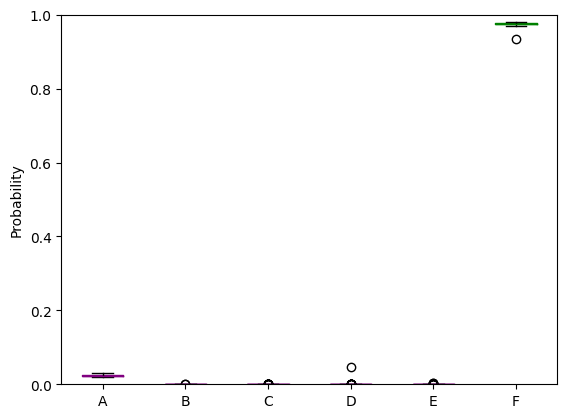
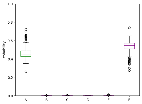
We can plot two instances where the BNN was correct, and two where it was not correct.

plt.rcParams["figure.figsize"] = (6.4, 4.8)

## two correct prediction
corr_0 = boxplot_model_predictions(prob_predictions, c_in[107*200], test_label, run_ensemble = True)
corr_1 = boxplot_model_predictions(prob_predictions, c_in[75*200], test_label, run_ensemble = True)

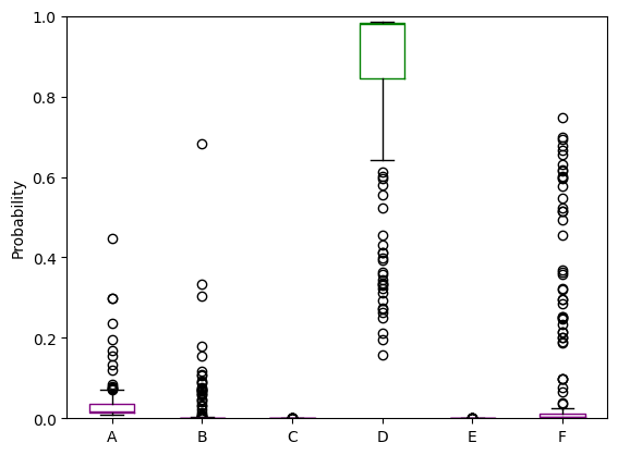
## two incorrect predictions
incorr_0 = boxplot_model_predictions(prob_predictions, inc_in[100], test_label, run_ensemble = True)
incorr_1 = boxplot_model_predictions(prob_predictions, inc_in[200], test_label, run_ensemble = True)

# Note in these box and whisker plots the distributions themselves represent the aleatoric uncertainty
# and the box and whiskers (ie. the ensemble of possible distributions) represent the epistemic uncertainty

------------------------------
True cluster: F

------------------------------
Model estimated probabilities:

_images/7de1f0813111d4208096cdad8357cbccc3da2d9c43b2a4900bf2f4d683d92d80.png

------------------------------
True cluster: D

------------------------------
Model estimated probabilities:

_images/82b39e76aba677395c3eb39ebd726f9fe3a4c1f67bb9340828b7b1d58b53339e.png

------------------------------
True cluster: C

------------------------------
Model estimated probabilities:

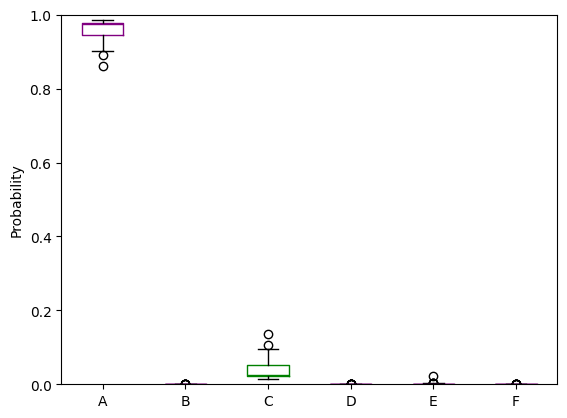
_images/443ac650d5e38d8143e804b7c2f808732075f3a52ff01baa7337572db37376fb.png

------------------------------
True cluster: A

------------------------------
Model estimated probabilities:

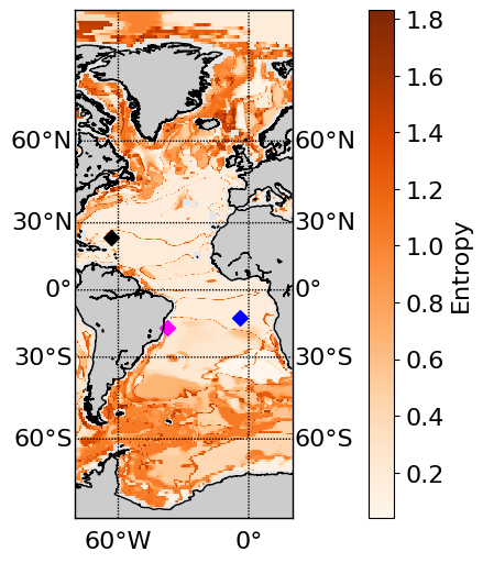
_images/bf77066b3e30c78ae321d3e9e4f4be4d2ea51b81cd73e395607810461d0b46e6.png

Entropy#

Model uncertainty can be quantified by calculating the entropy of the distribution. The higher the value, the more unsure the model is. The following code plots the entropy on a map.

! pip install Basemap # note you may have this already installed and therefore do not need to run this line

from mpl_toolkits.basemap import *

plt.rcParams.update({'font.size': 16})

entropy = -np.sum(prob_mean* np.log2(prob_mean), axis=1)
all_results = np.nan * np.zeros((360*720))
all_results[maskTest.flatten()] = entropy
lat = monthly_ssh['lat']
lon = monthly_ssh['lon']
lons = lon[1,:].values
lats = lat[:,1].values
llons, llats = np.meshgrid(lons,lats)
fig, ax = plt.subplots(figsize = (12, 6))
m = Basemap(llcrnrlon=-80, urcrnrlon=20, llcrnrlat=-80, urcrnrlat=89, projection='mill', resolution='l')
m.drawmapboundary(fill_color='0.9')
m.drawparallels(np.arange(-90.,99.,30.),labels=[1,1,0,1])
m.drawmeridians(np.arange(-180.,180.,60.),labels=[0,0,0,1])
m.drawcoastlines()
m.fillcontinents()
im1 = m.pcolor(llons, llats, np.flipud(np.reshape(all_results,(360,720)))[::-1,:], latlon=True, cmap = plt.cm.Oranges)
cbar = plt.colorbar(pad=0.075)
cbar.set_label('Entropy')
im2 = m.scatter([-63.25], [23.75], marker = 'D', c = 'black',  s = 50, latlon = True)
im3 = m.scatter([-4.25], [-12.75], marker = 'D', c = 'blue',  s = 50, latlon = True)
im4 = m.scatter([-37.25], [-17.25], marker = 'D', c = 'magenta', s = 50, latlon = True)
plt.show()

_images/d596b93dec32da9d5d42ac0009b8d7bd51c18fc9543d7d49e0bc8c2196a88842.png

plot_entropy_distribution(prob_mean, Y_test)

32610
7718

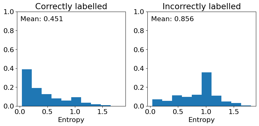
_images/c0430a0ced59be2f168766ffc71b71b1ea81a71eb5039c474eb1e0ceefeaaa5a.png

This shows that indeed, the entropy is higher on average for incorrect classifications than for correct ones.

There are also many other interesting plots that can be produced from BNN predictions as shown in Clare et al. 2022. The code to make these plots is at the end of this notebook on github