Global Air Quality Index

Global Air Quality Index#

Run the tutorial via free cloud platforms:

Learning objectives#

In this notebook we’ll compute the forecasts of the global air quality index (AQI). The computation of the AQI forecast is based on the forecast concentration of the following pollutants: \(O_3, NO_2, SO_2, PM2.5, PM10\). The index is computed according to the European Air Quality Index definition. The concentration of the pollutants will be time averaged and transformed in \(\mu g \cdot m^{-3}\) and finally classified in one of six levels, from Good to Extremly poor, according to the threshold levels defined in the European Air Quality Index. The air quality index is the highest value of the concentration levels of the pollutants. For instance, if the concentration level in a grid cell for \(NO_2, SO_2, PM2.5, PM10\) is Good but for \(O_3\) is Mediocre, then the air quality index for that grid cell is Mediocre.

Initial setup#

Before we begin we must prepare our computing environment. This includes installing the client software of the Application Programming Interface (API) of the Climate Data Store (CDS), intalling all the packages required to execute the code, setting up our CDS API credentials and importing the various Python libraries that will be used. If you are executing this notebook on your laptop it is assumed that you have created a conda environment with all the packages installed as specified in the environment.yml file in the root folder of the repository. On the other hand, if you are using a cloud environment, such as Google Colab, you will have to uncomment the following cell to install those packages since they are not provided by default.

# If you are running this notebook in Colab, ensure that the cdsapi package is installed
#!pip install -q cdsapi

# If you are running this notebook in Colab, uncomment the line below and run this cell.
#!pip install cartopy

# If you are running this notebook in Colab, uncomment the line below and run this cell
#!pip install xarray==2024.7.0

Add your ADS API credentials#

To set up your ADS API credentials, please login/register on the ADS, then you will see your unique API key in your profile.

You can copy your API key to your current session by replacing ######### in the code cell below

import os
os.environ['CDSAPI_URL'] = 'https://ads.atmosphere.copernicus.eu/api'
os.environ['CDSAPI_KEY'] = '###########################################'

Import libraries#

import numpy as np
import pandas as pd
import xarray as xr
import matplotlib
import matplotlib.pyplot as plt
import matplotlib.colors as mcol
from matplotlib import cm, ticker
from matplotlib.colors import ListedColormap
import cartopy
import cartopy.crs as ccrs
import cartopy.feature as cfeature
import seaborn as sns
from zipfile import ZipFile
import cdsapi
import warnings
warnings.filterwarnings('ignore')
from platform import python_version
print('Python version: %s'%python_version())
print('NumPy version: %s'%np.version.version)
print('Pandas version: %s'%pd.__version__)
print('Xarray version: %s'%xr.__version__)
print('Matplotlib version: %s'%matplotlib.__version__)
print('Cartopy version: %s'%cartopy.__version__)
print('Seaborn version: %s'%sns.__version__)

Python version: 3.12.5
NumPy version: 2.0.2
Pandas version: 2.2.2
Xarray version: 2024.7.0
Matplotlib version: 3.9.2
Cartopy version: 0.23.0
Seaborn version: 0.13.2

Here we specify a data directory in which we will download our data and all output files that we will generate:

DATADIR = '.'

Explore and download data#

We use the CAMS global atmospheric composition forecasts dataset. The spatial resolution is lower than that available for the CAMS European air quality forecasts used in the previous edition of the training event but it covers the whole planet. The dataset is available from the Copernicus Atmosphere Monitoring Service (CAMS). The spatial grid is 0.4° x 0.4° so that each cell has size 44 km x 44 km, approximately. In order to compute the air quality index for each grid cell we will download the data of the pollutants and the meteorological data: surface pressure, and 2m air temperature. The trace gases are provided for 137 vertical levels and are available at 3-hours intervals. We will download the trace gases data only for the surface level, that is level 137. The particulate matter and the meteorological data are available at a single level (surface) at hourly intervals.

Ozone mass mixing ratio [kg kg**-1]
Sulphur dioxide mass mixing ratio [kg kg**-1]
Nitrogen dioxide mass mixing ratio [kg kg**-1]
Particulate matter d <= 2.5 um [kg m**-3]
Particulate matter d <= 10 um [kg m**-3]
Surface pressure [Pa]
2m air temperature [K]

The concentration of the trace gases is given using a dimensionless unit. Since we want to use a common unit for all the pollutants we will have to transform the trace gases data from a dimensionless unit to mass concentration. We will use the surface pressure and the air temperature to perform such transformation. We will request the forecast data for 96 hours, 4 days, starting from the current day at time 00:00

Manual download#

The Copernicus Atmosphere Monitoring Service provides a user interface to select the dataset and the variables of interest and download the data from their website, in addition to the APIs. This option is useful in order to have an understanging of what variables are included in a dataset and how to build a request. The web page allows a user to copy the code to submit a request using the APIs. We can visit the download form for the CAMS global forecast data and select the variables of interest. We select in the “Single level” panel

2m temperature
surface pressure
Particulate matter d < 2.5 µm (PM2.5)
Particulate matter d < 10 µm (PM10)

In the “Multi level” panel, we select

Nitrogen dioxide
Ozone
Sulphur dioxide

In the “Model level” panel we select 137 (ground level)

For the date, we may select the current date for both start and end date. For the “Time”, that is the hour of the beginning of the forecasts we may select 00:00.

In the “Leadtime hour” panel we can flag all the check boxes from 0 to 95 for a 4 days forecast.

At the end of the download form, select Show API request. This will reveal a block of code, which contains the same settings as the code cells for the APIs download that we will use in the API download.

Please remember to accept the terms and conditions at the bottom of the download form.

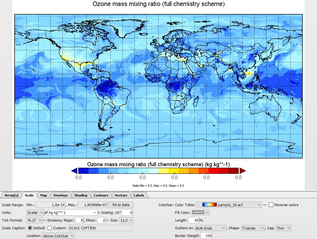
You might want to have a look at the content of the dataset using a NetCDF visualization tool such as Panoply

global O3

API download#

Once we have a better knowledge of the dataset, which names are used for our variables of interest, and the forecast days and times, we can set up a request to be sent through the CDS APIs

start_date = '2024-10-03'
end_date = '2024-10-03'
init_hour = '00'
lead_time_start = 0
lead_time_stop = 96
step_hours = 1
leadtime_hours = list(range(lead_time_start, lead_time_stop + lead_time_start, step_hours))

variables = ['2m_temperature',
            'surface_pressure', 
            'particulate_matter_2.5um',
            'particulate_matter_10um',
            'nitrogen_dioxide', 
            'ozone',
            'sulphur_dioxide']
bb_north = 90
bb_south = -90
bb_west = -180
bb_east = 180
area = [bb_north, bb_west, bb_south, bb_east]  

dataset = 'cams-global-atmospheric-composition-forecasts'

request = {
        'variable': variables,
		'date': f'{start_date}/{end_date}',
        'time': f'{init_hour}:00',
        'leadtime_hour': leadtime_hours,
        'model_level': '137',
        'type': 'forecast',
        'area': area,
        'format': 'netcdf_zip'
    }

c = cdsapi.Client()
c.retrieve(
    dataset,
    request,
    f'{DATADIR}/download.zip')

2024-10-04 09:51:16,228 WARNING [2024-10-04T07:51:15.581596] You are using a deprecated API endpoint. If you are using cdsapi, please upgrade to the latest version.
2024-10-04 09:51:16,229 INFO Request ID is 09f66ddd-7a47-466a-ae5f-a7857662a3d8
2024-10-04 09:51:16,268 INFO status has been updated to accepted
2024-10-04 09:51:17,804 INFO status has been updated to running
2024-10-04 09:52:30,516 INFO status has been updated to successful

'./download.zip'

We open the zip file to extract the NetCDF data files. Trace gases concentrations are in the multi-level variable file data_mlev.nc. The particulate matter concentrations and the meteorological variables, 2m air temperature and surface pressure, are in the single level variables file data_sfc.nc.

with ZipFile(f'{DATADIR}/download.zip', 'r') as zipObj:
   zipObj.extractall(path=f'{DATADIR}/')

We can remove the zip file

os.remove(f'{DATADIR}/download.zip')

Unit transformation#

We calculate the scaling factor to convert the dimensionless mixing ratios of \(NO_2, SO_2\), and \(O_3\) from kg/kg to mass density in ug/m3, using the air surface pressure and the temperature. The scaling factor c is defined as

\[c = \frac{p}{R_aT}\]

where \(R_a\) is the gas constant of dry air, p the pressure and T the temperature. The derivation of the scalar factor is provided in the appendix.

R = 287.08
cfactor = single_level_ds['sp'] / (R * single_level_ds['t2m'])

With the scaling factor we can transform the concentration values of the trace gases into \(kg \cdot m^{-3}\), the same unit used for the particulate matter. Then, we multiply for \(10^9\) to represent the values in \(\mu g \cdot m^{-3}\)

trace_gases = ['no2','go3','so2']
for gas in trace_gases:
    multi_level_ds[gas] = multi_level_ds[gas] * cfactor * 1e9

particulate_matter = ['pm2p5','pm10']
for param in particulate_matter:
    single_level_ds[param] = single_level_ds[param] * 1e9

Plotting the global concentrations forecasts of trace gases and particulate matter#

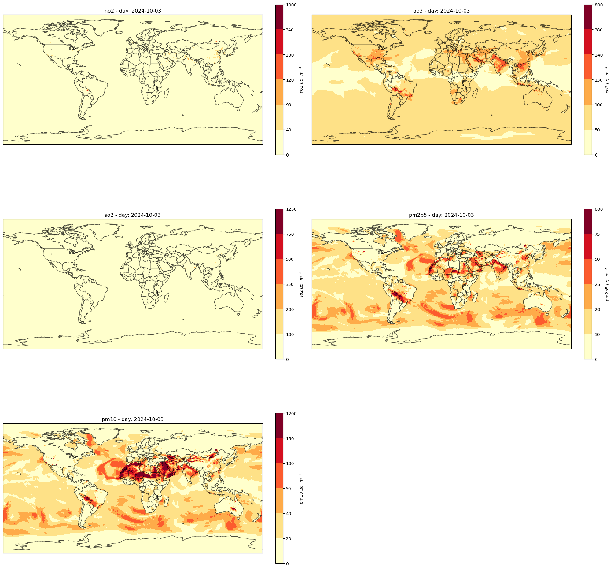
We plot the forecasts for the concentrations of the five pollutants for one day. We can plot any of the other forecast day by simply changing its day index (from 0 to 3)

params = ['no2','go3','so2','pm2p5','pm10']

We define the levels of the pollutants to be plotted in order to map the values within each interval using a predefined colormap. We use different levels for each pollutant according to the concentration levels defined for the European Air Quality Index.

no2_limits = [0, 40, 90, 120, 230, 340, 1000]
o3_limits = [0, 50, 100, 130, 240, 380, 800]
so2_limits = [0, 100, 200, 350, 500, 750, 1250]
pm25_limits = [0, 10, 20, 25, 50, 75, 800]
pm10_limits = [0, 20, 40, 50, 100, 150, 1200]

all_levels = [no2_limits, o3_limits, so2_limits, pm25_limits, pm10_limits]

day_index = 0 # index of the daily forecasts, from 0 to 3
fig, axs = plt.subplots(nrows=3, ncols=2,
                        subplot_kw={'projection': ccrs.PlateCarree()},
                        figsize=(20, 20), layout='constrained') 
axs = axs.flatten()
days = [str(day)[:10] for day in eaqi_daily.valid_time.to_numpy()]
fig.delaxes(axs[5])
for i, param in enumerate(params):
    da = eaqi_daily[param]
    clevs = all_levels[i]
    day = days[day_index]
    data = da[day_index,:,:] 
    cs = axs[i].contourf(da.longitude, da.latitude, data, 
                        levels = clevs, 
                        cmap='YlOrRd', # 'RdYlBu_r', 
                        norm = mcol.BoundaryNorm(clevs, 256), 
                        transform=ccrs.PlateCarree())

    cbar = plt.colorbar(cs, fraction=0.046, pad=0.05, orientation='vertical', shrink=0.75, ticks=clevs)
    cbar.set_label(param + ' $\mu g \cdot m^{-3}$')
    #axs[i].set_yticklabels(clevs)
    axs[i].set_extent([bb_west, bb_east, bb_south, bb_north], crs=ccrs.PlateCarree()) 
    axs[i].set_title(param + ' - day: ' + day)
    axs[i].coastlines(color='black', alpha=0.7) 
    axs[i].add_feature(cfeature.LAKES, alpha=0.7, edgecolor='black', facecolor='none')
    axs[i].add_feature(cfeature.BORDERS, alpha=0.7)
    axs[i].margins(0.1)

_images/5779f5ec84d0bbc484cd3b4f00e1eb28e8dc98bfa031ee401162057306236eb6.png

Calculating the air quality index#

With the concentration of the five polluttants we can calculate the air quality index. The air quality index of a pollutant X can be calculated using the equation

\[I_x = \frac{I_{high} - I_{low}}{C_{high} - C_{low}}(C_x - C_{low}) + I_{low}\]

where \(I_{high}\) is the right AQI index value of the interval that contains the concentration value \(C_x\), \(I_{low}\) is the left AQI index value, and \(C_{low}\) and \(C_{high}\) are the concentration thresholds of that interval.

\(NO_2\) \((\mu g/m^3)\)	\(O_3\) \((\mu g/m^3)\)	\(SO_2\) \((\mu g/m^3)\)	\(PM2.5\) \((\mu g/m^3)\)	\(PM10\) \((\mu g/m^3)\)	AQI	Category
0-40	0-50	0-100	0-10	0-20	1	Good
40-90	50-100	100-200	10-20	20-40	2	Fair
90-120	100-130	200-350	20-25	40-50	3	Moderate
120-230	130-240	350-500	25-50	50-100	4	Poor
230-340	240-380	500-750	50-75	100-150	5	Very Poor
340-1000	380-800	750-1250	75-800	150-1200	6	Extremely Poor

We use the same intervals defined for the European Air Quality Index to compute the value of the index from the concentration values of the pollutant

bin_list = all_levels

We define a function to map the concentration values to one of the intervals that have been defined for the air quality index

def classify_forecast_variables(forecast_ds):
    '''
    This function assigns an integer value according to a class 
    for each float value in the dataset.
    '''
    classified_arrays = []
    for i in range(0, len(forecast_ds)):
        variable = params[i]
        temp = xr.apply_ufunc(np.digitize,
                              forecast_ds[variable],
                              bin_list[i])
        classified_arrays.append(temp)
        combined_arrays = xr.merge(classified_arrays)
        final_index = combined_arrays.to_array().max('variable')
    return final_index

aqi_index = classify_forecast_variables(eaqi_daily)

We define a colormap for the AQI according to the EEA colourscale

good_color = '#03fcf0'
fair_color = '#16d984'
moderate_color = '#dffa11'
poor_color = '#db4918'
very_poor_color = '#873c23'
extremely_poor_color = '#5a2387'
colors = [good_color, fair_color, moderate_color, poor_color, very_poor_color, extremely_poor_color]
labels = ['Good', 'Fair', 'Moderate', 'Poor', 'Very Poor', 'Extremely Poor']
levels = [0.5, 1.5, 2.5, 3.5, 4.5, 5.5, 6.5]
level_ticks = [1, 2, 3, 4, 5, 6]
aqi_cmap = ListedColormap(colors)

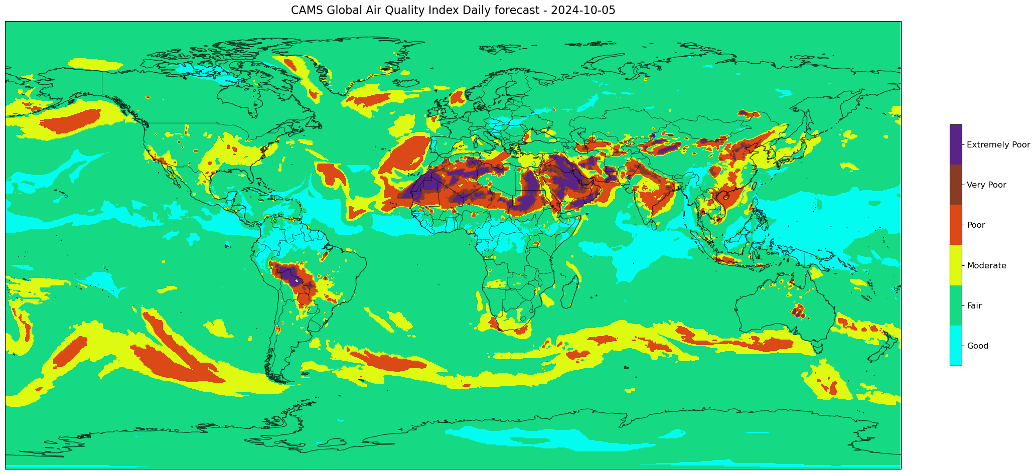
Global AQI map#

day = '2024-10-05'
fig, ax = plt.subplots(subplot_kw={'projection': ccrs.PlateCarree()},
                       figsize=(25, 25))
timestamp = aqi_index.valid_time
data = aqi_index.sel(valid_time=day)
cs=ax.contourf(aqi_index.longitude, 
                       aqi_index.latitude, 
                       data,
                       levels=levels, 
                       cmap=aqi_cmap,
                       transform=ccrs.PlateCarree())
    
ax.set_title('CAMS Global Air Quality Index Daily forecast - ' + day, fontsize=16, pad=10.0)
ax.coastlines(color='black', alpha=0.7, resolution='50m')
ax.add_feature(cfeature.BORDERS, alpha=0.7, linewidth=0.7)
ax.set_extent([bb_west, bb_east, bb_south, bb_north], crs=ccrs.PlateCarree())
    
# Customize colorbar
cbar = plt.colorbar(cs, fraction=0.028, pad=0.05, shrink=0.25) 
cbar.set_label(None)
cbar.ax.tick_params(labelsize=12)
cbar.set_ticks(level_ticks)
cbar.set_ticklabels(labels)

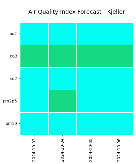
_images/c7ebd6681446a39337b3c4861549492b1ea41018658211e6572d1790389e5e2a.png

Air quality heatmap for Kjeller#

We can plot the air quality forecast of the polluttants as heatmap for any location by using its latitude and longitude. In this example we will plot the air quality forecast heatmap for Kjeller, a village east of Oslo, Norway. We will map the concentration of the polluttants in Kjeller to the classes defined for the air quality calculation. This step is similar to what was done before for the global map. After the ma

kjeller_lat = 59.9742
kjeller_lon = 11.0469

kjeller_day = eaqi_daily.sel(latitude = kjeller_lat, longitude = kjeller_lon, method='nearest')

days = [str(day)[:10] for day in kjeller_day.valid_time.to_numpy()]
days_index = pd.to_datetime(days)
days_index

DatetimeIndex(['2024-10-03', '2024-10-04', '2024-10-05', '2024-10-06'], dtype='datetime64[ns]', freq=None)

def classify_forecast(forecast_ds, bin_list):
    '''
    This function assigns an integer value according to a class 
    in the bin_list to each float value in the input dataset.
    The function returns a Pandas series.
    '''
    classified_arrays = []
    temp = xr.apply_ufunc(np.digitize,
                          forecast_ds,
                          bin_list)
    classified_arrays.append(temp)
    combined_arrays = xr.merge(classified_arrays)
    aqi_index = combined_arrays.to_array().max('variable')
    aqi_ds = aqi_index.to_series()
    return aqi_ds.values

kjeller_no2 = classify_forecast(kjeller_day['no2'], no2_limits)
kjeller_o3 = classify_forecast(kjeller_day['go3'], o3_limits)
kjeller_so2 = classify_forecast(kjeller_day['so2'], so2_limits)
kjeller_pm25 = classify_forecast(kjeller_day['pm2p5'], pm25_limits)
kjeller_pm10 = classify_forecast(kjeller_day['pm10'], pm10_limits)

kjeller_dict = {'pm10': kjeller_pm10,
                'pm25': kjeller_pm25,
                'so2': kjeller_so2,
                'o3': kjeller_o3,
                'no2': kjeller_no2}

kjeller_df = pd.DataFrame(kjeller_dict, index=days_index)
kjeller_df

	pm10	pm25	so2	o3	no2
2024-10-03	1	1	1	2	1
2024-10-04	1	2	1	2	1
2024-10-05	1	1	1	2	1
2024-10-06	1	1	1	2	1

kjeller_df = (kjeller_df.T).iloc[::-1]
kjeller_df

	2024-10-03	2024-10-04	2024-10-05	2024-10-06
no2	1	1	1	1
o3	2	2	2	2
so2	1	1	1	1
pm25	1	2	1	1
pm10	1	1	1	1

fig, ax = plt.subplots(1, 1, figsize=(5, 5))
#cbar_ax = fig.add_axes([.82, .13, .01, .75])
#fig.tight_layout()
g = sns.heatmap(kjeller_df, 
                cmap=aqi_cmap, 
                linewidth = 0.5, 
                linecolor = 'w', 
                ax=ax,
                #cbar_ax = cbar_ax, 
                vmin = 1, 
                vmax = 6, cbar=False)

g.set_title("\nAir Quality Index Forecast - Kjeller\n", fontsize=14)
#g.set(xlabel=None)

g.set_yticklabels(params, fontsize=10, rotation=0)

xlabels = kjeller_df.columns.format('%Y-%m-%d')[1::]
g.set_xticklabels(xlabels, fontsize=10);

# Customize colorbar entries
#cbar = ax.collections[0].colorbar  
#cbar.set_ticks([1.4,2.2,3.1,3.9,4.8,5.6])
#cbar.set_ticklabels(labels)
#cbar.ax.tick_params(labelsize=11)

_images/95f3e3fa206432da22be1e608732ae3771cf48c3035bc1e0cf2160cf96b38357.png

References#

Jacob - Introduction to Atmospheric Chemistry
Wilks - Statistical Methods in Atmospheric Science, 2nd Edition

Appendix - Scaling factor#

We start from the definition of mass mixing ratio of a chemical species X in air

\[\alpha_x = \frac{\rho_x}{\rho}\]

where \(\rho_x\) is the mass density of the chemical species X in \(kgm^{-3}\) and \(\rho\) is the mass density of the air. We assume the trace gases and the dry air to follow the ideal gas law so that for dry air we can write

\[pV = nRT\]

where p is the air pressure, \(R = K_B N_A = 8.314 \text{ } JK^{-1}mol^{-1}\) is the ideal gas constant, where \(K_B\) is the Boltzmann constant and \(N_A\) is the Avogadro’s number, V the volume, T the temperature, and finally n is the number of moles. The number of moles is defined as the ratio of the mass and the molar mass. For dry air, a mixture of several gases, the molar mass \(M_a\) can be represented by the weighted sum of the molar masses of all the chemical species in the air (see Jacob, chap.1, p.4)

\[M_a = \sum_i w_iM_i = 28.96 \cdot 10^{-3} \text{ } kg\text{ }mol^{-1}\]

With this defnition the number of moles of dry air can be written as

\[n = \frac{m}{M_a}\]

where m is the mass of the dry air. Substituting this definition into the gas law for dry air we have

\[pV = \frac{m}{M_a}RT\]

We can define the gas constant of dry air from the ideal gas constant R and the molar mass of dry air

\[R_a = \frac{R}{M_a} = \frac{8.314 \text{ } JK^{-1}mol^{-1}}{28.96 \cdot 10^{-3} \text{ } kg\text{ }mol^{-1}} = 287.08 \text{ } JK^{-1}kg^{-1}\]

We can now write the law for dry air as

\[pV = mR_aT\]

and

\[p = \frac{m}{V}R_aT = \rho R_aT\]

so that the mass density of dry air is

\[\rho = \frac{p}{R_aT}\]

from which we can write the equation of the mass density of a chemical species in the air as a function of its mixing ratio, the air pressure and temperature, and given the air specific gas constant

\[\rho_x = \alpha_x \frac{p}{R_aT} \text{ } kg m^{-3}\]

If we define the factor c as