Tutorial on comparing CARRA and ERA5 2m temperature data¶

This notebook can be run on free online platforms, such as Binder, Kaggle and Colab, or they can be accessed from GitHub. The links to run this notebook in these environments are provided here, but please note they are not supported by ECMWF.

Introduction¶

Understanding global and regional atmospheric conditions is critical for climate research, weather forecasting, and environmental monitoring. Reanalysis datasets like ERA5 (ECMWF’s fifth-generation global reanalysis) and CARRA (Copernicus Arctic Regional Reanalysis) provide high-quality, gridded estimates of atmospheric variables, enabling scientists to study past weather and climate patterns. Both datasets can be found in, and are freely accessible through, the Copernicus Climate Data Store (CDS).

Both datasets enhance our insights into Earth’s systems, but they are different in several aspects. ERA5 offers a comprehensive global perspective with a resolution of approximately 31 km. Meanwhile CARRA is regional and tailored for the Arctic region, delivering higher spatial resolution (~2.5 km) and specialized insights into polar processes, that make it particularly adequate for studying the Arctic’s unique climate dynamics.

In this tutorial, we focus on comparing 2m temperature data from both datasets. There are 5 CARRA entries available in the CDS: sub-daily data for single, height, pressure and model levels and data aggregated for a day or month. Practical details of the CARRA dataset are available in the documentation. Meanwhile, the complete ERA5 portfolio of datasets is availble at ERA5.

Here the CARRA single level entry is selected for the 2m temperature. The ERA5 dataset, available in full via the Copernicus Climate Data Store (CDS), serves as our global benchmark. By comparing these datasets, you will get an awareness of their strengths, limitations, and potential applications — whether for validating regional models, assessing climate trends, or supporting decision-making in Arctic-sensitive sectors.

Learning objectives 🎯¶

This tutorial demonstrates how to access and retrieve CARRA and ERA5 data and how to inter-compare them on the CARRA domain. CARRA is a high resolution (2.5 km) regional re-analysis which gives added details compared to the ERA5 global reanalysis. These details can be visualised by comparing the plots of CARRA and ERA5 data, and particularly when the differences of the two datasets are plotted together. By the end, you will have:

Accessed and downloaded 2m temperature data from both the ERA5 and CARRA data, interacting with the Copernicus Climate Data Store using Python code.
Prepared the data for an inter-comparison, by interpolating them to the same grid and computing monthly means.
Created engaging map-like visuals (plots), that emphasize the differences between the two datasets.

Prepare your environment¶

The first thing we need to do, is make sure you are ready to run the code while working through this notebook. There are some simple steps you need to do to get yourself set up.

Set up CDSAPI and your credentials¶

The code below will ensure that the cdsapi package is installed. If you have not setup your ~/.cdsapirc file with your credentials, you can replace None with your credentials that can be found on the how to api page (you will need to log in to see your credentials).

!pip install -q cdsapi
# If you have already setup your .cdsapirc file you can leave this as None
cdsapi_key = None
cdsapi_url = None

(Install and) Import libraries¶

To run the code in this tutorial please install any missing packages here.

Please note that the package xESMF is not in the environment file, but can be installed following the instructions here.

import os
import cdsapi
import warnings
import cdsapi
import matplotlib.pyplot as plt
import cartopy.crs as ccrs
import xarray as xr
# Package to interpolate ERA5 data to the CARRA grid
import xesmf as xe

warnings.filterwarnings('ignore') #turn off some warnings

Specify data directory¶

# Directory to store data
DATADIR = './data_dir/'
# Create this directory if it doesn't exist
os.makedirs(DATADIR, exist_ok=True)


period="202403" # the period to plot
fCARRA = os.path.join(DATADIR,"carra_T2m_an_"+period+".grb")
fERA5 = os.path.join(DATADIR,"era5_T2m_an_"+period+".grb")

Explore data¶

The source code will download a specific month. By specifying the start and end date below, one can easily download longer periods. We are selecting 2m temperature, which is in the single level CDS entry. Here, we download the 3-hourly analysis time steps, and the data will be stored in a specified file.

For this tutorial we just request one month of data, March 2024. Note that we define a sub-domain to use for the ERA5 request.

# Here one specifies the domain, year and period to download

yearStart = 2024 #first year to download
yearEnd   = 2024 #last year to download
monthStart =  3 # first month to download
monthEnd   =  3 #last month to download
days = [str(i).zfill(2) for i in range(1,31)] # the list of days to download. Adapt day number for other months
domain = 'west_domain' # the domain to select. Use "east_domain" for the CARRA-East domain
period="202403" # the period to plot

# Below a polygon to limit the area downloaded from ERA5, otherwise it will download the whole world
area_for_era5 = [90, -110, 55, 40] #WEST domain polygon, format: North,West,South,East corners
#area_for_era5 = [85,0,60,50]: EAST domain polygon

Download the data¶

Define helper functions to formulate the CDS data request¶

The functions below allow repeated CDS API requests to be made, in case multiple requests are required to retrieve high volumes of data. In this case we are only requesting one month.

# Call the CDS client
c = cdsapi.Client(url=cdsapi_url,key=cdsapi_key)

# Define a helper function to download the data
# Note that the time is hardcoded since we are selecting
# all possible available times. 
def fetch_month_carra(month, year, days, domain, fout):
    c.retrieve(
        'reanalysis-carra-single-levels',
        {
            'format': 'grib',
            'domain': domain ,
            'level_type': 'surface_or_atmosphere',
            'variable': '2m_temperature',
            'product_type': 'analysis',
            'year': year,
            'month': month,
            'day': days,
            'time': [
                '00:00', '03:00', '06:00',
                '09:00', '12:00', '15:00',
                '18:00', '21:00',
            ],
        },
        fout)
    
# Help function to download ERA5 data
def fetch_month_era5(month, year, days, area, fout):
    c.retrieve(
    'reanalysis-era5-single-levels',
    {
        'product_type': 'reanalysis',
        'variable': '2m_temperature',
        'year': str(year),
        'month': str(month).zfill(2),
        'day': days,
        'time': [
            '00:00', '03:00', '06:00',
            '09:00', '12:00', '15:00',
            '18:00', '21:00',
        ],
        'area': area,
        'format': 'grib',
    },
     fout)

Request the CARRA-West data¶

The loops below may be useful if you are requesting a large volume of data, in this case one month is being requested.

# Loop through the period selected (in this example only 2024 03 is requested)
for year in list(range(yearStart, yearEnd + 1)):
    for month in list(range(1,13)):
        if year == yearStart and month < monthStart:
            # Before the start date.
            continue
        if year == yearEnd and month > monthEnd:
            # After end date.
            break

        print ("CARRA data will be fetched for ", year, month)
        print("This will take a few minutes, depending on the data size (here ~621 MB for west, ~357 MB for east case)")
        fetch_month_carra(month, year, days, domain,fCARRA)

Request the ERA5 data¶

# Loop through the period selected
for year in list(range(yearStart, yearEnd + 1)):
    for month in list(range(1,13)):
        if year == yearStart and month < monthStart:
            # Before the start date.
            continue
        if year == yearEnd and month > monthEnd:
            # After end date.
            break

        print ("ERA5 data will be fetched for ", year, month)
        print("This will take a few minutes, depending on the data size (here ~39 MB for west area)")
        fetch_month_era5(month, year, days, area_for_era5,fERA5)

Plotting the CARRA and ERA5 data¶

Interpolate data to a common grid¶

Before plotting the two datasets we want to have them on the same grid. For this we interpolate ERA5 to the CARRA (CARRA-West) grid. Below we use xesmf. The interpolation/projection can also be done using the pyresample library, or CDO.

Inspect the ERA5 datacube.

ERA5  = xr.open_dataset(fERA5)
ERA5

Inspect the CARRA datacube.

CARRA  = xr.open_dataset(fCARRA)
CARRA

We remove some additional coordinates in the datasets, to ease the regridding operation.

ERA5 = ERA5.drop_vars(['number', 'step', 'valid_time', 'surface'])
CARRA = CARRA.drop_vars(['step', 'valid_time', 'heightAboveGround'])

Now use xesmf bilinear interpolation to construct a regridder object and apply it to the ERA5 data.

# Create regridder using xesmf bilinear interpolation
regridder = xe.Regridder(ERA5, CARRA, "bilinear")
# Regrid the data
print("regridding the ERA5 data")
ERA5_CARRA = regridder(ERA5)
print("done")

Check the format of the output and save it.

ERA5_CARRA
fERA5_CARRA_grid = os.path.join(DATADIR,"era5_t2m_"+period+"_CARRA_grid.nc")
ERA5_CARRA.to_netcdf(fERA5_CARRA_grid)

Plotting the data¶

Compute the mean 2m temperature over the whole month. First, we open the data sets using xarray and then calculate their mean over the whole month, prepare the dataset for plotting on a latitude/longitude grid, and the temperature units (from Kelvin to degrees Celsius).

# Open the data sets to plot using xarray

import xarray as xr

# Open Datasets
CARRA = xr.open_dataset(fCARRA)
CARRA = CARRA.drop_vars(['step', 'valid_time', 'heightAboveGround'])
ERA5  = xr.open_dataset(fERA5_CARRA_grid)

# Compute monthly mean
print("Computing the mean for CARRA and ERA5...")
CARRA_mean = CARRA.mean("time", keep_attrs=True)
ERA5_mean = ERA5.mean("time", keep_attrs=True)
print("Done.")

# Change longitudes from 0-360 to -180 to 180, needed for the plotting
CARRA_mean = CARRA_mean.assign_coords(longitude=(((CARRA_mean.longitude + 180) % 360) - 180))
ERA5_mean = ERA5_mean.assign_coords(longitude=CARRA_mean.longitude)

# Change unit from K to C and add the unit to the attributes
CARRA_mean_C = CARRA_mean - 273.15
CARRA_mean_C = CARRA_mean_C.assign_attrs(CARRA_mean.attrs)
CARRA_mean_C.attrs['units'] = 'deg C'
ERA5_mean_C = ERA5_mean - 273.15
ERA5_mean_C = ERA5_mean_C.assign_attrs(ERA5_mean.attrs)
ERA5_mean_C.attrs['units'] = 'deg C'

Plot for CARRA¶

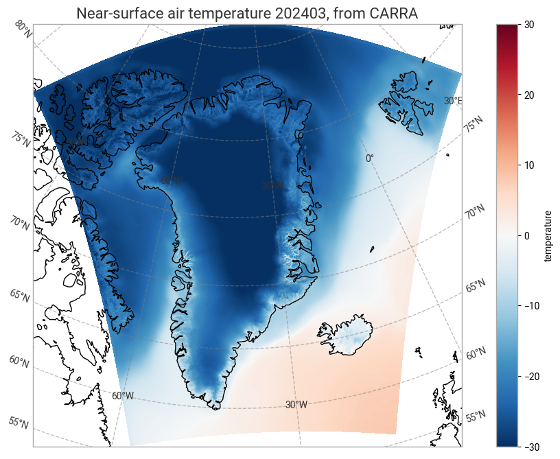
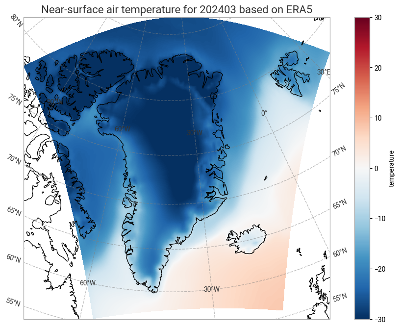
We fix the scale of each of the separate CARRA and ERA5 plots to the range from -30 to 30 degrees Celsius. This ensures the two figures can be compared directly.

The plot below shows the CARRA 2m temperature monthly mean (March 2024) values for the CARRA-West domain.

print("Plotting CARRA mean surface temperature")
# Create the figure panel and the map using the Cartopy Lambert conformal projection
fig, ax = plt.subplots(1, 1, figsize = (16, 8), subplot_kw={'projection': ccrs.LambertConformal(central_latitude=70.0, central_longitude=-40.0)})

# Plot the data
im = plt.pcolormesh(CARRA_mean_C.longitude, CARRA_mean_C.latitude,CARRA_mean_C.t2m,
                    transform = ccrs.PlateCarree(), cmap='RdBu_r', vmin=-30, vmax=30)

# Set the figure title
ax.set_title('Near-surface air temperature '+period+', from CARRA', fontsize=16)
ax.coastlines(color='black')
ax.gridlines(draw_labels=True, linewidth=1, color='gray', alpha=0.5, linestyle='--') 

# Specify the colourbar
cbar = plt.colorbar(im,fraction=0.05, pad=0.04)
cbar.set_label('temperature')

Plotting CARRA mean surface temperature

Plot for ERA5¶

The plot shows ERA5 2m temperature monthly mean (March 2024) values on the CARRA-West domain.


print("Plotting ERA5 mean surface temperature")

# Create the figure panel and the map using the Cartopy Lambert conformal projection
fig, ax = plt.subplots(1, 1, figsize = (16, 8), subplot_kw={'projection': ccrs.LambertConformal(central_latitude=70.0, central_longitude=-40.0)})

# Plot the data
im = plt.pcolormesh(ERA5_mean_C.longitude, ERA5_mean_C.latitude, ERA5_mean_C.t2m, 
                    transform = ccrs.PlateCarree(), cmap='RdBu_r', vmin=-30, vmax=30)

# Set the figure title
ax.set_title('Near-surface air temperature for '+period+' based on ERA5', fontsize=16)
ax.coastlines(color='black')
ax.gridlines(draw_labels=True, linewidth=1, color='gray', alpha=0.5, linestyle='--') 

# Specify the colourbar
cbar = plt.colorbar(im,fraction=0.05, pad=0.04)
cbar.set_label('temperature')

Plotting ERA5 mean surface temperature

Plot the difference between CARRA and ERA5¶

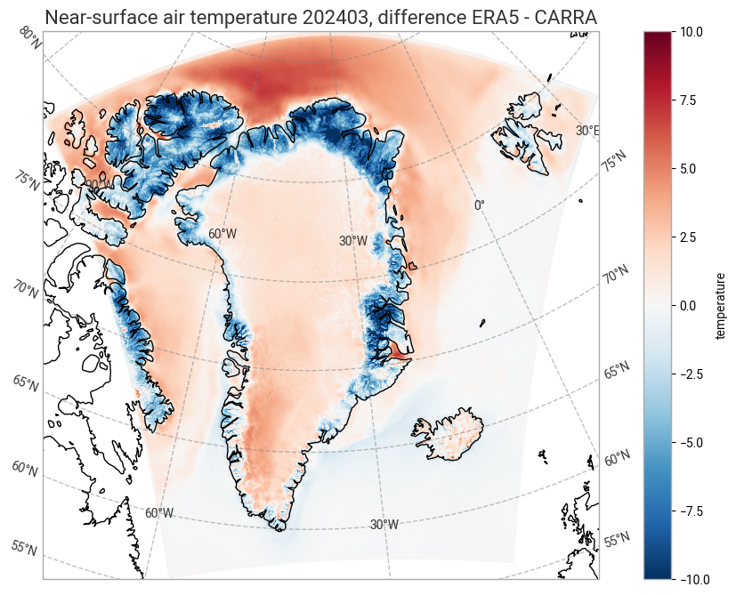
Note that the differences are computed in the plotting command itself. Here we plot the difference with a range of -10 to 10 degrees Celsius.

The plot shows the 2m monthly mean (March 2024) 2m temperature difference between CARRA and ERA5 over the CARRA-West domain.

print("Plot the difference CARRA - ERA5")
# Create the figure panel and the map using the Cartopy Lambert conformal projection
fig, ax = plt.subplots(1, 1, figsize = (16, 8), subplot_kw={'projection': ccrs.LambertConformal(central_latitude=70.0, central_longitude=-40.0)})

# Plot the data, the differences are computed directly in the line below.
im = plt.pcolormesh(CARRA_mean_C.longitude, CARRA_mean_C.latitude, ERA5_mean_C.t2m - CARRA_mean_C.t2m,
                    transform = ccrs.PlateCarree(), cmap='RdBu_r', vmin=-10, vmax=10)

# Set the figure title
ax.set_title('Near-surface air temperature '+period+', difference ERA5 - CARRA', fontsize=16)
ax.coastlines(color='black')
ax.gridlines(draw_labels=True, linewidth=1, color='gray', alpha=0.5, linestyle='--') 

# Specify the colourbar
cbar = plt.colorbar(im,fraction=0.05, pad=0.04)
cbar.set_label('temperature')

Plot the difference CARRA - ERA5

Take home messages 📌¶

CARRA and ERA5 data, while broadly similar, contain subtle, but important differences in values due to their spatial scope. These differences are important to note.
Note the differences visible between CARRA and ERA5, especially over coastal areas and over complex orography (mountainous terrain) where the high resolution CARRA data can provide additional information compared to ERA5, such as for instance the significantly lower temperatures at higher elevations near the coasts.
The differences in northern ocean areas likely come from the better description of sea-ice characteristics by CARRA.
The differences are much easier to see in the difference plot above, however they can also be recognised in the individual plots as finer details in the CARRA plot.