CHALLENGE: Compute the latitudinally weighted mean over space and time for the NUTS regions - ECMWF internal earthkit training, March 2026

Challenge notebook: content/earthkit-transforms/02c-spatial-challenge.ipynb

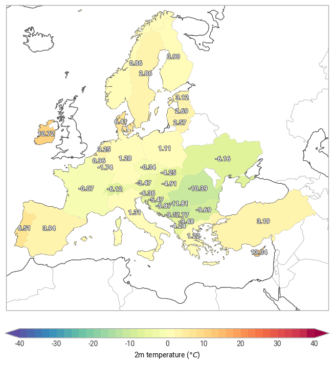
Provide the additional arguments to the ekt.spatial.reduce method to compute the latitudinally weighted mean, over space and time, for the nuts_regions. The answer should look like this:

For me details and hints, see the Reducing data-cubes using geometry objects tutorial.

from earthkit import data as ekd
from earthkit import geo as ekg
from earthkit import plots as ekp
from earthkit import transforms as ekt
from earthkit.transforms._tools import earthkit_remote_test_data_file

Load some data¶

In this example we will use hourly ERA5 2m temperature data on a 0.5x0.5 spatial grid for the year 2015 as our physical data; and we will use the NUTS regions geometries which are available in earthkit.geo.

# NUTS regions
nuts_data = ekg.gisco.nuts_regions(level=0).to_geopandas()
nuts_data.head()

remote_era5_file = earthkit_remote_test_data_file("era5_temperature_europe_20150101.grib")
era5_data = ekd.from_source("url", remote_era5_file)
# Convert to xarray, we keep all time steps for the challenge
era5_xr = era5_data.to_xarray(time_dims=["valid_time"]).rename({"2t": "t2m"})
era5_xr

Reduce data¶

reduced_data = ekt.spatial.reduce(
    era5_xr,
    nuts_data,
    mask_dim="NAME_ENGL",
    how="mean",  # Default value
    # INSERT EXTRA KWARGS HERE TO REDUCE ALSO IN THE TIME DIMENSION,
    # AND TO WEIGHT THE MEAN WITH LATITUDE
)

# Add the reduced data back to the original GeoDataFrame for plotting
nuts_data = nuts_data.assign(t2m=reduced_data.t2m)

Plot the data using earthkit.plots.geo.choropleth.

fig = ekp.geo.choropleth(
    nuts_data,
    z="t2m",
    domain="Europe",
    metadata={"units": "K", "long_name": "2m temperature"},
    units="celsius",
    labels="{t2m:0.2f}",
)
fig.coastlines()
fig.borders()
fig.show()