Reducing data-cubes over geometries - ECMWF internal earthkit training, March 2026

from earthkit import data as ekd
from earthkit import geo as ekg
from earthkit import plots as ekp
from earthkit import transforms as ekt
from earthkit.transforms._tools import earthkit_remote_test_data_file

Load some test data¶

In this example we will use hourly ERA5 2m temperature data on a 0.5x0.5 spatial grid for the year 2015 as our physical data; and we will use the NUTS regions geometries which are available in earthkit.geo.

# NUTS regions
nuts_data = ekg.gisco.nuts_regions(level=0).to_geopandas()
nuts_data.head()

remote_era5_file = earthkit_remote_test_data_file("era5_temperature_europe_20150101.grib")
era5_data = ekd.from_source("url", remote_era5_file)
# Convert to xarray and select the first time step for plotting
era5_xr = era5_data.to_xarray(time_dims=["valid_time"]).rename({"2t": "t2m"}).isel(valid_time=0)
era5_xr

Reduce data¶

reduced_data = ekt.spatial.reduce(
    era5_xr,
    nuts_data,
    mask_dim="NAME_ENGL",
    how="mean",  # Default value
)
reduced_data

Now we add the temperature data to the geopandas for easier plotting.

nuts_data = nuts_data.assign(t2m=reduced_data.t2m)
nuts_data.head()

Below we plot the geopandas dataframe using the geo.choropleth method in earthkit.plots.

fig = ekp.geo.choropleth(
    nuts_data,
    z="t2m",
    domain="Europe",
    metadata={"units": "K", "long_name": "2m temperature"},
    units="celsius",
    labels="{t2m:0.2f}",
)
fig.coastlines()
fig.borders()
fig.show()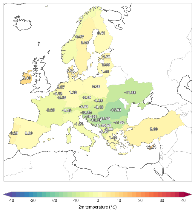

<earthkit.plots.components.figures.Figure at 0x13583aa20>