Climatology calculations - ECMWF internal earthkit training, March 2026

from earthkit import data as ekd
from earthkit import plots as ekp
from earthkit import transforms as ekt
from earthkit.transforms._tools import earthkit_remote_test_data_file

Get some demonstration ERA5 data, this could be any url or path to an ERA5 grib or netCDF file.

remote_era5_file = earthkit_remote_test_data_file("ERA5-Reading-2m-temperature-1940-2025.nc")
era5_xr = ekd.from_source("url", remote_era5_file).to_xarray()
era5_xr

Calculate the climatologies¶

The climatology module offers a range of methods for calculating climatological statistics. First we will use the basic methods to calculate climatological mean and standard-deviation representative of the climatology period 1991-2020.

The climatology_range must provide the start and end date for the climatology period. It can be provided as date strings which are recognised by xarray, for example "YYYY", "YYYY-MM" and "YYYY-MM-DD", or as a date objects such as datetime objects or numpy.datetime64 objects.

If the climatology range is not provided, then the whole time-period in the input data is used.

climatology_mean = ekt.climatology.mean(era5_xr, climatology_range=("1991", "2020"))
climatology_std = ekt.climatology.std(era5_xr, climatology_range=("1991", "2020"))
print(
    f"Climatology mean = {float(climatology_mean.t2m)}\nClimatology standard deviation = {float(climatology_std.t2m)}"
)

Climatology mean = 283.6854248046875
Climatology standard deviation = 5.9290385246276855

Monthly and daily climatologies¶

It is possible to calculate monthly and daily climatological statistics using the methods described in the API reference guide

The monthly/daily climatologies provide a value of the requested statistic for each calendar-month/day-of-year over the climatology_range period.

In the examples below, we calculate the monthly and daily mean for our 2m temperature data for the climatology_range 1990 to 2020. In the returned objects the valid_time dimension has been replaced with a month/dayofyear dimension.

climatology_monthly_mean = ekt.climatology.monthly_mean(era5_xr, climatology_range=("1991", "2020"))
climatology_monthly_mean

climatology_daily_mean = ekt.climatology.daily_mean(era5_xr, climatology_range=("1991", "2020"))
climatology_daily_min = ekt.climatology.daily_min(era5_xr, climatology_range=("1991", "2020"))
climatology_daily_max = ekt.climatology.daily_max(era5_xr, climatology_range=("1991", "2020"))
climatology_daily_mean

Plot the output¶

First we plot the climatology data using an earthkit-plots Climatology figure.

chart = ekp.Climatology(wrap_time=True)

chart.fix_y_units("celsius")

# Daily mean + min/max envelope
chart.line(
    climatology_daily_mean,
    label="Daily mean",
    color="cornflowerblue",
)
chart.fill_between(
    climatology_daily_min,
    climatology_daily_max,
    label="Daily min/max range",
    color="cornflowerblue",
)
chart.line(
    climatology_monthly_mean,
    label="Monthly mean",
    color="seagreen",
    lw=2,
)
chart.title(
    "Daily and monthly climatology for {variable_name}\n{location:%c}, {location:%C} ({latitude:%Lt}, {longitude:%Ln})"
)
chart.xticks(frequency="M", period=True)
chart.ylabel()
chart.legend()
chart.show()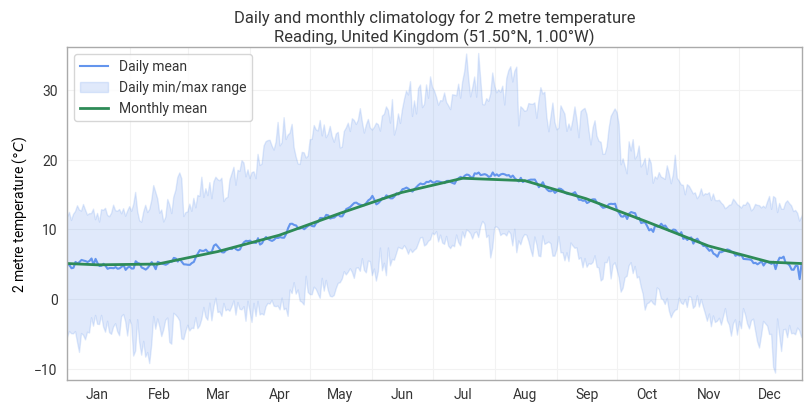

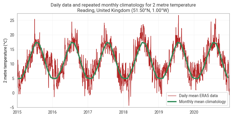
Now we add the climatology to the background of the Timeseries plot for the daily mean on the original valid_time dimension. First we create the repeated climatology for the monthly quantiles, then we plot with earthkit-plots

latitude = 51.5
longitude = -1.0

chart = ekp.TimeSeries()

era5_daily_mean = ekt.temporal.daily_mean(era5_xr)
chart.line(
    era5_daily_mean.sel(valid_time=slice("2015", "2020")),
    units="celsius",
    label="Daily mean ERA5 data",
    color="firebrick",
    lw=1,
)

# repeat_years tiles the month-dimensioned climatology across 2015–2017
# automatically — no dummy datetime coordinates needed.
chart.line(
    climatology_monthly_mean,
    units="celsius",
    label="Monthly mean climatology",
    color="seagreen",
    lw=3,
    repeat_years=range(2015, 2021),
)

chart.title(
    "Daily data and repeated monthly climatology for {variable_name}\n"
    "{location:%c}, {location:%C} ({latitude:%Lt}, {longitude:%Ln})"
)
chart.ylabel()
chart.legend()
chart.show()