This short how-to guides you through the steps to create a timeseries of the agricultural land fraction using CORINE land cover data and save it as a csv file. The final csv file can be used as, e.g., exposure data for the drought risk estimation.
We use CORINE land cover data from the Copernicus Land Monitoring Service, which provides harmonized land cover maps for 1990, 2000, 2006, 2012, and 2018.
Settings
User settings
admin_id = "EL64" # Example admin ID for Central GreeceSetup of environment
import xarray as xr
import numpy as np
import pandas as pd
import geopandas as gpd
import regionmask
from pathlib import Path
import rioxarray as rxr
import os
import re

# Set up data directories
data_dir = Path("../data")
corine_dir = data_dir / "corine_landcover"

print(f"\nCORINE data directory: {corine_dir}")
CORINE data directory: ../data/corine_landcover
Setup region specifics
# Read NUTS shapefiles
regions_dir = data_dir / 'regions'
nuts_shp = regions_dir / 'NUTS_RG_20M_2024_4326' / 'NUTS_RG_20M_2024_4326.shp'
nuts_gdf = gpd.read_file(nuts_shp)

# Select the region of interest
sel_gdf = nuts_gdf[nuts_gdf['NUTS_ID'] == admin_id]
print(f"Found {admin_id} region: {sel_gdf['NUTS_NAME'].values[0]}")
print(f"Bounding box: {sel_gdf.geometry.total_bounds}")
lon_min, lat_min, lon_max, lat_max = sel_gdf.geometry.total_bounds

# Create a regionmask from the admin region geometry
admin_mask = regionmask.from_geopandas(sel_gdf, names='NUTS_ID')
Found EL64 region: Στερεά Ελλάδα
Bounding box: [21.39637798 37.98898161 24.67199242 39.27219519]
Define CORINE land cover classes
# CORINE Land Cover class names (official nomenclature)
corine_classes = {
    # Artificial surfaces (1-11)
    1: 'Continuous urban fabric', 2: 'Discontinuous urban fabric',
    3: 'Industrial or commercial units', 4: 'Road and rail networks',
    5: 'Port areas', 6: 'Airports', 7: 'Mineral extraction sites',
    8: 'Dump sites', 9: 'Construction sites', 10: 'Green urban areas',
    11: 'Sport and leisure facilities',
    # Agricultural areas (12-22)
    12: 'Non-irrigated arable land', 13: 'Permanently irrigated land',
    14: 'Rice fields', 15: 'Vineyards', 16: 'Fruit trees and berry plantations',
    17: 'Olive groves', 18: 'Pastures', 19: 'Annual crops associated with permanent crops',
    20: 'Complex cultivation patterns', 21: 'Land principally occupied by agriculture',
    22: 'Agro-forestry areas',
    # Forest and semi-natural areas (23-34)
    23: 'Broad-leaved forest', 24: 'Coniferous forest', 25: 'Mixed forest',
    26: 'Natural grasslands', 27: 'Moors and heathland', 28: 'Sclerophyllous vegetation',
    29: 'Transitional woodland-shrub', 30: 'Beaches, dunes, sands',
    31: 'Bare rocks', 32: 'Sparsely vegetated areas', 33: 'Burnt areas',
    34: 'Glaciers and perpetual snow',
    # Wetlands (35-39)
    35: 'Inland marshes', 36: 'Peat bogs', 37: 'Salt marshes',
    38: 'Salines', 39: 'Intertidal flats',
    # Water bodies (40-44)
    40: 'Water courses', 41: 'Water bodies', 42: 'Coastal lagoons',
    43: 'Estuaries', 44: 'Sea and ocean'
}

# Define land cover class groups
agricultural_classes = list(range(12, 23))  # Classes 12-22
forest_classes = list(range(23, 30))  # Classes 23-29
urban_classes = list(range(1, 12))  # Classes 1-11
water_classes = list(range(40, 45))  # Classes 40-44

print(f"Total CORINE classes: {len(corine_classes)}")
print(f"Agricultural classes (12-22): {len(agricultural_classes)} types")
Total CORINE classes: 44
Agricultural classes (12-22): 11 types
Download CORINE land cover data
The CORINE land cover data is downloaded manually through the Copernicus Land Monitoring Service: https://
In the viewer, select the CORINE land cover data for all years available (1990, 2000, 2006, 2012, 2018). To reduce the amount of data, you can limit the spatial extent to your administrative region (e.g., NUTS-2 region “Central Greece” - EL64).
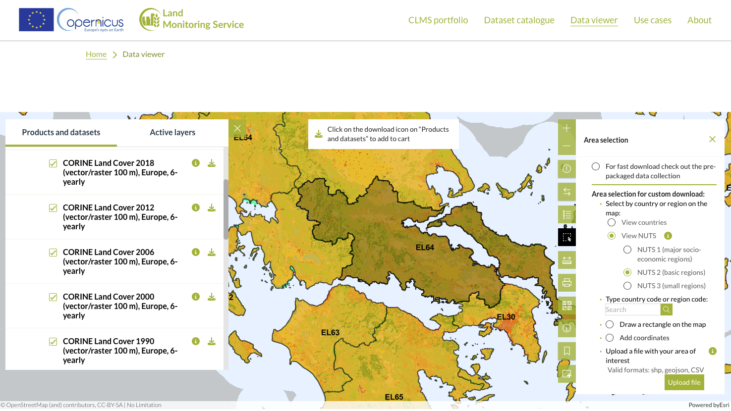
For each dataset year, add it to the cart and select:
Format: Raster
Projection: EPSG:4326 (WGS84)
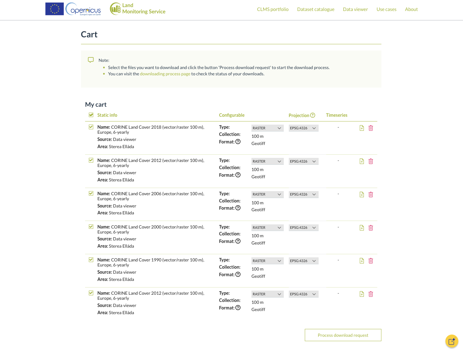
Once downloaded, move the data into the following subdirectory:
./data/corine_landcover/Process data for the region
Read raw data
# List all CORINE tif files
tif_files = list(corine_dir.glob("*/*/*.tif"))
print(f"Found {len(tif_files)} CORINE tif files:")
for f in tif_files:
    print(f"  {f.name}")
Found 5 CORINE tif files:
U2000_CLC1990_V2020_20u1.tif
U2006_CLC2000_V2020_20u1.tif
U2012_CLC2006_V2020_20u1.tif
U2018_CLC2018_V2020_20u1.tif
U2018_CLC2012_V2020_20u1_raster100m.tif
# Read all tif files into a single xarray dataset
datasets = []
years = []

for tif_file in tif_files:
    # Read using rioxarray
    ds = rxr.open_rasterio(tif_file)

    # Extract year from filename - look for pattern like CLC1990, CLC2000, etc.
    year_match = re.search(r'CLC(\d{4})', tif_file.name)
    if year_match:
        year = int(year_match.group(1))
        years.append(year)
        print(f"Processing year: {year}")
    else:
        print(f"Warning: Could not extract year from {tif_file.name}")
        continue

    datasets.append(ds)

# Sort datasets and years together by year
sorted_pairs = sorted(zip(years, datasets), key=lambda x: x[0])
years, datasets = zip(*sorted_pairs)

# Concatenate along new time dimension
corine_ds = xr.concat(datasets, dim="time")
corine_ds = corine_ds.rename({"band": "land_cover", "x": "lon", "y": "lat"})

# Assign time based on extracted years
corine_ds["time"] = pd.to_datetime([f"{year}-01-01" for year in years])
corine_ds = corine_ds.assign_coords(time=corine_ds.time)
corine_ds = corine_ds.squeeze("land_cover")  # remove land_cover dimension

# Replace fill value (-128) with NaN
corine_ds = corine_ds.where(corine_ds != -128)

print(f"\nCORINE dataset shape: {corine_ds.shape}")
print(f"Years available: {years}")
print(f"Coordinate ranges: lon=[{float(corine_ds.lon.min()):.2f}, {float(corine_ds.lon.max()):.2f}], lat=[{float(corine_ds.lat.min()):.2f}, {float(corine_ds.lat.max()):.2f}]")
Processing year: 1990
Processing year: 2000
Processing year: 2006
Processing year: 2018
Processing year: 2012
CORINE dataset shape: (5, 1650, 3105)
Years available: (1990, 2000, 2006, 2012, 2018)
Coordinate ranges: lon=[21.26, 24.79], lat=[37.93, 39.43]
Calculate grid cell areas
Calculate the area of each grid cell, accounting for variations by latitude.
# Calculate grid cell areas (accounting for latitude)
# Earth radius in meters
R = 6371000

# Get lat/lon spacing
lat = corine_ds.lat.values
lon = corine_ds.lon.values
dlat = np.abs(np.diff(lat).mean())
dlon = np.abs(np.diff(lon).mean())

# Calculate area for each latitude (in km²)
lat_rad = np.deg2rad(lat)
# Area = R² * dλ * (sin(φ₂) - sin(φ₁))
areas = R**2 * np.deg2rad(dlon) * np.abs(
    np.sin(lat_rad + np.deg2rad(dlat/2)) -
    np.sin(lat_rad - np.deg2rad(dlat/2))
) / 1e6  # Convert to km²

# Create 2D area array
area_2d = np.tile(areas[:, np.newaxis], (1, len(lon)))

print(f"Grid cell areas range from {areas.min():.2f} to {areas.max():.2f} km²")
print(f"Total study area: {area_2d.sum():.2f} km²")
Grid cell areas range from 0.01 to 0.01 km²
Total study area: 51199.45 km²
Calculate coverage of broad land cover categories
# Calculate land cover percentages for each year
def calculate_coverage(data_array, class_list, area_2d):
    """Calculate areal coverage for specified classes"""
    mask = np.isin(data_array.values, class_list)
    total_area = area_2d[~np.isnan(data_array.values)].sum()
    class_area = area_2d[mask & ~np.isnan(data_array.values)].sum()
    return (class_area / total_area) * 100

results = []
for i, year in enumerate(corine_ds.time.dt.year.values):
    data = corine_ds.isel(time=i)

    # Calculate percentages for major categories
    agri_pct = calculate_coverage(data, agricultural_classes, area_2d)
    forest_pct = calculate_coverage(data, forest_classes, area_2d)
    urban_pct = calculate_coverage(data, urban_classes, area_2d)
    water_pct = calculate_coverage(data, water_classes, area_2d)

    results.append({
        'year': year,
        'agricultural': agri_pct,
        'forest': forest_pct,
        'urban': urban_pct,
        'water': water_pct
    })

    print(f"{year}: Agricultural={agri_pct:.1f}%, Forest={forest_pct:.1f}%, Urban={urban_pct:.1f}%, Water={water_pct:.1f}%")

df_coverage = pd.DataFrame(results)
print("\nLand cover categories:")
print(df_coverage)
1990: Agricultural=33.3%, Forest=62.7%, Urban=1.3%, Water=1.1%
2000: Agricultural=33.3%, Forest=62.5%, Urban=1.5%, Water=1.1%
2006: Agricultural=32.4%, Forest=62.4%, Urban=2.2%, Water=1.1%
2012: Agricultural=31.8%, Forest=62.5%, Urban=2.6%, Water=1.1%
2018: Agricultural=31.7%, Forest=62.4%, Urban=2.6%, Water=1.1%
Land cover categories:
year agricultural forest urban water
0 1990 33.279219 62.715590 1.252794 1.067083
1 2000 33.257153 62.504301 1.510422 1.055861
2 2006 32.446728 62.442879 2.181934 1.109056
3 2012 31.755714 62.452383 2.562456 1.105405
4 2018 31.745346 62.425693 2.620222 1.105405
Calculate coverage of agricultural categories
# Detailed breakdown of agricultural land by crop type
agri_class_names = {
    12: 'Non-irrigated arable', 13: 'Permanently irrigated',
    14: 'Rice fields', 15: 'Vineyards', 16: 'Fruit trees',
    17: 'Olive groves', 18: 'Pastures', 19: 'Annual+permanent crops',
    20: 'Complex cultivation', 21: 'Agriculture+natural',
    22: 'Agro-forestry'
}

agri_breakdown = []
for i, year in enumerate(corine_ds.time.dt.year.values):
    data = corine_ds.isel(time=i)
    row = {'year': year}

    for cls in agricultural_classes:
        pct = calculate_coverage(data, [cls], area_2d)
        row[agri_class_names[cls]] = pct

    agri_breakdown.append(row)

df_agri = pd.DataFrame(agri_breakdown)
print("Agricultural land breakdown:")
print(df_agri)
Agricultural land breakdown:
year Non-irrigated arable Permanently irrigated Rice fields Vineyards \
0 1990 9.675677 3.523386 0.103912 0.095955
1 2000 9.678976 3.548181 0.072627 0.097757
2 2006 5.558817 7.323455 0.230085 0.091398
3 2012 5.307652 7.742775 0.228292 0.098860
4 2018 5.304568 7.733826 0.228292 0.098860
Fruit trees Olive groves Pastures Annual+permanent crops \
0 0.163262 4.380540 0.291327 0.104831
1 0.163391 4.374450 0.288768 0.104831
2 0.144353 4.734827 0.349343 0.104831
3 0.143172 5.271346 0.368523 0.100512
4 0.144966 5.271346 0.369299 0.100512
Complex cultivation Agriculture+natural Agro-forestry
0 6.282549 8.657781 0.0
1 6.244557 8.683615 0.0
2 5.813614 8.096005 0.0
3 5.582367 6.912215 0.0
4 5.582367 6.911311 0.0
Save regional data
Save regional coverage timseries to CSV
# Create output directory
output_dir = data_dir / admin_id / "corine_land_cover"
output_dir.mkdir(parents=True, exist_ok=True)

# Save main land cover categories
csv_file_main = output_dir / "land_cover_categories.csv"
df_coverage.to_csv(csv_file_main, index=False)
print(f"Saved main land cover categories to: {csv_file_main}")

# Save agricultural land breakdown
csv_file_agri = output_dir / "agricultural_land_breakdown.csv"
df_agri.to_csv(csv_file_agri, index=False)
print(f"Saved agricultural land breakdown to: {csv_file_agri}")
Saved main land cover categories to: data/EL64/corine_land_cover/land_cover_categories.csv
Saved agricultural land breakdown to: data/EL64/corine_land_cover/agricultural_land_breakdown.csv
Save spatial raster (latest year)
# Save the most recent year as GeoTIFF for use in tutorial
latest_year_idx = -1
latest_data = corine_ds.isel(time=latest_year_idx)
latest_year = int(corine_ds.time.dt.year.values[latest_year_idx])

# Set spatial dimensions and CRS for rioxarray
latest_data = latest_data.rio.set_spatial_dims(x_dim='lon', y_dim='lat')
latest_data.rio.write_crs("EPSG:4326", inplace=True)

# Save as GeoTIFF
tif_file = output_dir / f"corine_landcover_{admin_id}.tif"
latest_data.rio.to_raster(tif_file, driver="GTiff")
print(f"Saved processed {latest_year} CORINE land cover raster to: {tif_file}")
Saved processed 2018 CORINE land cover raster to: data/EL64/corine_land_cover/corine_landcover_EL64.tif
Output summary
Output files created:
land_cover_categories.csv- Timeseries of main land cover categories (agricultural, forest, urban, water)agricultural_land_breakdown.csv- Timeseries of detailed agricultural land typescorine_landcover_{admin_id}.tif- Spatial raster of CORINE land cover (latest year)
These files can now be used in the agricultural land tutorial for visualization and analysis.