Looking at Sea Level and derived Surface Current data¶

This notebook can be run on free online platforms, such as Binder, Kaggle and Colab, or they can be accessed from GitHub. The links to run this notebook in these environments are provided here, but please note they are not supported by ECMWF.

Introduction¶

Gridded sea level data from satellite observations for the global ocean from 1993 to present provides sea surface height values, measured using radar altimetry satellites. The sea level dataset provided through the C3S Climate Data Store is climate-oriented, that is, dedicated to the monitoring of the long-term evolution of sea level and the analysis of the ocean/climate indicators, both requiring a homogeneous and stable sea level record. To achieve this, a steady two-satellite merged constellation is used at all time steps in the production system: one satellite serves as reference and ensures the long-term stability of the data record; the other satellite (which varies across the record) is used to improve accuracy, sample mesoscale processes and provide coverage at high latitudes.

The C3S sea level dataset is used to produce Ocean Monitoring Indicators such as the mean sea level evolution, an important climate indicator, available in the Copernicus Marine Environment Monitoring Service (CMEMS) catalogue. Stability is also of importance when considering kinetic energy evolution in the ocean, as the addition of a satellite in the input data can add details in surface currents from which this quantity is computed, thus apparently changing the kinetic energy.

Learning objectives 🎯¶

This notebook-tutorial provides a practical introduction to the Sea level gridded data from satellite observations for the global ocean from 1993 to present data, available through the Climate Data Store (CDS). These datasets contain data for the Sea Level Essential Climate Variable (ECV), as well as Surface Currents (the latter only in the daily dataset). We give a short introduction to the Sea level data and to their derived surface currents. We provide two use cases of the datasets:

• plot the monthly Sea Level data during an El Niño event (Use Case 1), and

• plot the Sea Level and derived parameters over a strong current (Use Case 2).

We provide step-by-step instructions and each line of code is explained.

Prepare your environment¶

The first thing we need to do, is make sure you are ready to run the code while working through this notebook. There are some simple steps you need to do to get yourself set up.

Set up CDSAPI and your credentials¶

The code below will ensure that the cdsapi package is installed. If you have not setup your ~/.cdsapirc file with your credentials, you can replace None with your credentials that can be found on the how to api page (you will need to log in to see your credentials).

(Install and) Import libraries¶

The data have been stored in files written in NetCDF format. To best handle these, we will import the Xarray library which is specifically designed for manipulating multidimensional arrays in the field of geosciences. The libraries Matplotlib and Cartopy will also be imported for plotting and visualising the analysed data. We will also import the libraries zipfile to work with zip-archives, OS to use OS-functions and pattern expansion, and urllib3 for disabling warnings for data download via CDS API.

Specify data directory¶

Explore data¶

Satellite radar altimetry measures the distance between the satellite sensor and the water (or ice) surface, also called “range”. Several independent instruments onboard the satellites provide information on the satellite altitude, which enables a sea surface height to be computed with respect to either the reference ellipsoid (a geometric surface approximating Earth surface), the geoid (an equipotential of the Earth gravity field), or a mean sea surface (thus including only variable heights) by subtracting the range from the altitude.

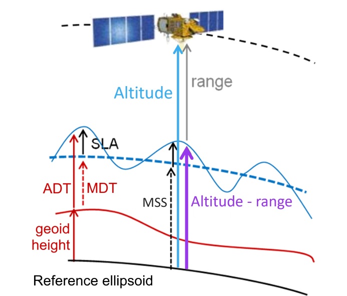
Figure 1. Scheme of altimetry principle, to provide with the different names which will be used later on.

Acronyms and concepts used in this notebook (and any content dealing with sea level data from altimetry), referred to in Figure 1:

• SLA Sea Level Anomaly (sea surface height with respect to a mean sea surface) represents ocean variability (sometimes called SSHA).

• ADT Absolute Dynamic Topography (sea surface height with respect to the geoid) represents the heights linked to everything moving in the ocean, including the stable currents (often named ‘sea surface height’ by oceanographers, but this name is ambiguous without a reference given).

• MSS Mean Sea Surface is a multi-year average of the sea surface heights with respect to a reference ellipsoid -- MSS is not provided in the C3S data.

• MDT Mean Dynamic Topography : ADT = SLA + MDT ; MDT is obtained through MSS - geoid and also drifter current velocity analysis. It represents the heights linked to the mean stable currents. It is now provided through CMEMS as an independent dataset.

• EKE Eddy Kinetic Energy: the kinetic energy computed from the geostrophic currents derived from the slope of the sea level anomalies.

In the ocean, surface topography gradients are related to pressure gradients and therefore to currents through geostrophy.

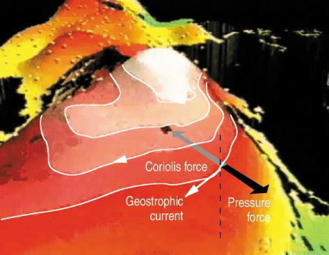
Figure 2. Geostrophic currents around a (positive) relief in the sea surface height. These currents are generated by the balance between the horizontal pressure gradient forces exerted by water masses and the effect of acceleration due to the Earth’s rotation (Coriolis’ force).

Those currents are computed from derivatives of the sea surface height slope (either SLAs or ADTs; it can also be done with MDT heights). In the two different directions (zonal (longitude) component, meridional (latitude) component), the computation outside of the Equatorial area is:

And

with g the gravitational constant, f the Coriolis frequency.

In the +/- 5°N band (Equatorial area), the computation is also done in the dataset, but by using second derivatives.

Two variants of the dataset are provided in the CDS, Daily and Monthly mean, which do not include exactly the same variables (we will examine their respective contents later on in this tutorial):

• in the Sea Level gridded daily products, currents are provided as total geostrophic currents (ADT gradients: ugos and vgos) and geostrophic current anomalies (SLA gradients, ugosa and vgosa).

• In the Monthly Mean products, you will find the kinetic energy, which is computed from them, equal to ( 1/2 * $\sqrt{u^2 + v^2)}$ ), but not the eastwards (aka zonal) and northwards (aka meridional) components of the geostrophic currents separately.

Download the data¶

Please find further information about the datasets as well as the data in the Climate Data Store sections “Overview”, “Download data” and “Documentation”:

• Sea level gridded data from satellite observations for the global ocean from 1993 to present overview

• Sea level gridded data from satellite observations for the global ocean from 1993 to present download data

• Sea level gridded data from satellite observations for the global ocean from 1993 to present documentation

Use Cases¶

Use Case 1: Explore and plot a Monthly mean Gridded Sea Level file at the peak of an El Niño episode¶

Objectives:

• read the Sea Level Anomaly variable,

• overview what Sea Level Anomalies can show of the ocean dynamics,

• plot the Sea Level Anomalies.

First of all, we will get an overview of the data content by looking at its metadata. Then, we will examine Sea Level Anomalies by plotting the monthly-averaged global distribution. The data are stored in NetCDF format, and we will use the Xarray library to work with the data. We will then use Matplotlib and Cartopy to visualise the data.

We start by downloading a Monthly mean file from 2015/11, using the latest version of the data available as of this day (vDT2021).

Build the request we send to the CDS, by defining the dataset we are requesting, the “variable”, date(s) and version (everything you can select in the “download” page of the Climate Data Store for this given dataset can thus be defined). Note that in this case “variable” refers to the dataset variants, i.e., either “Daily” or “Monthly mean”. We only choose one file in this tutorial, but, by adding other year(s) and/or month(s) in the lists, you could download more. You can also try other months to plot them.

NetCDF is a self-described format, i.e. it includes information (“metadata”) to help describe and explain the data, such as explicit name (long_name), standardized name (standard_name), comment, units, min and max values, also default values, etc. Those information items are called “attributes”, and are specific to the file, or to each variable; they are mostly optional, but highly recommended; the “standardization” of the format makes some of them mandatory. It is part of Copernicus Services’ requirements.

We will list all the data variables defined within the file.

You see here two geophysical variables, “SLA” and “EKE”. Both have (time, latitude, longitude) as dimensions. “Time” has only one value since we have only one file with one date.

We will have a look at some of the attributes of the data: the standard name and unit of the provided variables (note that the variables in the list above can have or not those attributes).

The first information is the variable name that we will call in the next cell, to plot it. The Standard names are homogeneizing vocabulary. Variable units are of course necessary to know, especially when they are not the SI unit proper but multiples or submultiples (such as $cm^2/s^2$ here).

Read and load a data variable for monthly Product: Sea Level Anomalies¶

To load a data variable, we just call it by its name. Moreover, we need longitude and latitude to plot it on a map. Those are included in the file as “dimensions”, but can be called the same way (to list dimension, you can use “ds.dims”).

Plot the monthly data for Sea Level Anomaly for Nov. 2015¶

We will plot the Sea Level Anomalies in a “plate carree” projection (scale: longitude = latitude).

We are keeping the default colour scale minimum and maximum (i.e. the minimum and maximum value of the variable within the given file -- it could be different on another month). The lands are coloured in grey (lightgrey) and delimited by a 1-px line. We set the extent of the plot using the maximum and minimum longitude and latitude defined above. We add a colour scale (colorbar), and a title; here we put the unit of the scale in the title, in a 16-size font.

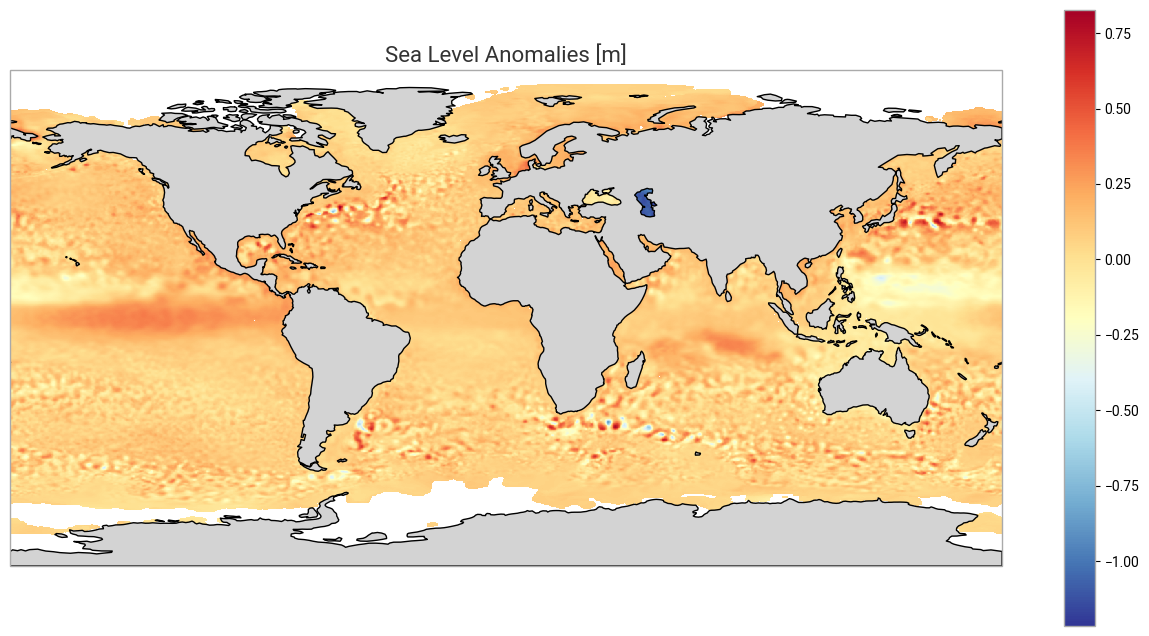
Figure 3. This plot shows the Sea Level Anomalies averaged for the month of November 2015. A lot of “dots” are present. Red and blue ‘dots’, mostly concentrated in the major current areas (e.g. the Gulf Stream, Antarctic Circumpolar Current, Kuroshio Current, among others) are strong mesoscale eddies, anticyclonic for “red” dots (higher-than-average sea level anomalies, also warm eddies), cyclonic for “blue” dots (lower-than-average sea level anomalies, also cold eddies). Some of those are present in this monthly average since they typically last for more than 30 days (they are moving, though, during such period). These eddies are an important part of vertical mixing of the ocean, and have thus a role in climate processes.

However, you may also have noticed a large structure West of South America, but it is cut by the projection centered on 0. We will see how to change the map centre, and look at that structure. Moreover, the whole map is somehow uniformly coloured, and not centered on 0 - defining the minimum and maximum of the colorbar used will improve the readability of the map.

Center the map on the Pacific, and define the colorbar extrema to better see what is happening.

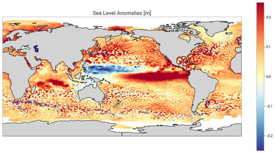
Figure 4. We see here better the higher-than-average sea level anomalies in the Eastern Tropical Pacific, which is one of the signatures of an El Niño episode (counterbalanced by lower-than-average sea level anomalies in the Western Pacific). If you look at the previous months, you will see this anomaly crossing the whole Pacific, from West to East, from Asia to South America.

Use case 2: Explore and plot a daily Gridded Sea Level file over the Gulf Stream area¶

Objectives:

• read different variables within a daily file,

• overview what those different variables can show concerning the ocean dynamics,

• compute a vector magnitude from its two components (current velocities),

• plot them.

Read and load a data variable for daily Product¶

We will open and explore a daily file, chosen on June 7, 2023 - the date is purely arbitrary, you can try another one from January 1st, 1993 to the latest available one (at the time of writing, June 7, 2023).

The beginning of the process is exactly the same as above, except the variant name (“variable”) of the dataset requested is now “daily”, and that we add a day in the month for the date.

Let’s see what data variables we have now - again, the instruction is the same as above, but not the resulting list.

You can see that they are more variables in this dataset variant. SLA is still here, but in the case of daily data, the EKE is not pre-computed. However, you have zonal (U) and meridional (V) components of the geostrophic velocity derived from the Sea Level Anomalies (ugosa, vgosa). You also have the absolute dynamic topography (ADT) and the corresponding geostrophic velocities (ugos, vgos). Let’s have a look at all those, and compute the current velocity as well, over the Gulf Stream area.

Select only the area and save the dataset thus created in a netcdf file for future uses.

Have a look at the extracted data structure as a whole:

Load the different sea surface height-related variables. First, we will plot the sea level anomalies (as for the monthly file) over our area of interest.

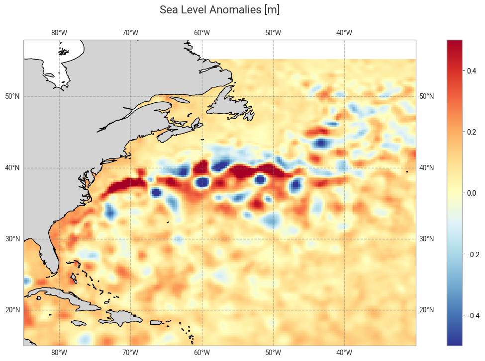
Figure 5. Sea Level Anomalies over the North-West Atlantic. The area with very high / very low “dots” (i.e., eddies) shows the turbulence of the Gulf Stream, with a number of eddies (and meanders of the current) thus visible. You may have noticed that we defined the minimum and maximum of the colorbar at lower/higher values than for the global monthly mean above, due to these higher/lower values.

Plot all the variables loaded or computed above, absolute dynamic topography (left) and anomalies (right), side by side.

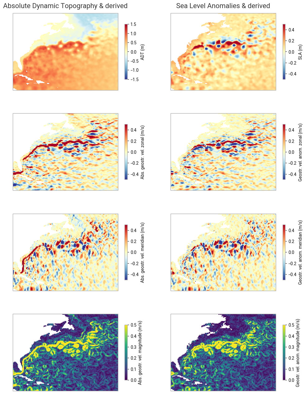
Figure 6. The top left map shows the sea surface heights (ADT) with respect to the geoid. One can see the “hill” (at North Atlantic basin’s scale!) which is the Gulf Stream gyre, around which the Gulf Stream system moves, clockwise. The first column shows the ADT and derived geostrophic velocities - U (i.e. eastward or “zonal” component) and V (i.e. Northward or “meridional” component), and the computation $\sqrt{u^2 + v^2)}$ , i.e. the current velocity (the vector magnitude). The second column shows the anomalies (notice the change in colorbar minimum & maximum between ADT and SLA). A large part is similar as in ADT since, in such an energetic current, turbulences constitute a major part of the dynamics, so eddies are of strong amplitude and clearly visible even upon the main flow of the current. However, in the bottom maps the main Gulf Stream flow is visible in the left map, as a large line coming from the Gulf of Mexico and continuing north-eastwards, while “only” rings and meanders are visible in the right map.

Take home messages 📌¶

In this tutorial, you have seen:

• how to retrieve, using the Climate Data Store, the different variants (monthly mean and daily) of the Sea level gridded data from satellite observations dataset,

• how to load those data so as to be able to use them, and what their respective contents are,

• what the Sea level gridded data variables mean with respect to ocean dynamics.

More information about Sea Level¶

• Sea level gridded data from satellite observations for the global ocean from 1993 to present overview

• Sea level gridded data from satellite observations for the global ocean from 1993 to present documentation

• About the Climate Data Store