Earthkit-hydro: Computing Accumulations Along River Networks¶

Tnis notebook will show a simple example of computing global and local accumulations along river networks.

import earthkit.data as ekd
import earthkit.plots as ekp
import earthkit.hydro as ekh

First, we load the relevant data needed for the notebook.

# load an example precipitation dataset
da = ekd.from_source(
    "sample",
    "R06a.nc",
).to_xarray()["R06a"].isel(time=0).load() # making sure it's not chunked in space
print(da)

# some nice custom plots styles
style = ekp.styles.Style(
    colors="Blues",
    levels=[0, 0.5, 1, 2, 5, 10, 50, 100, 500, 1000, 2000, 3000, 4000],
    extend="max",
)

# load the river network
network = ekh.river_network.load("efas", "5")

<xarray.DataArray 'R06a' (lat: 2970, lon: 4530)> Size: 54MB
array([[0.06744136, 0.06995939, 0.08337583, ...,        nan,        nan,
               nan],
       [0.0870114 , 0.08831516, 0.08961891, ...,        nan,        nan,
               nan],
       [0.11274368, 0.1154278 , 0.11811192, ...,        nan,        nan,
               nan],
       ...,
       [       nan,        nan,        nan, ..., 0.        , 0.        ,
        0.        ],
       [       nan,        nan,        nan, ..., 0.        , 0.        ,
        0.        ],
       [       nan,        nan,        nan, ..., 0.        , 0.        ,
        0.        ]], shape=(2970, 4530), dtype=float32)
Coordinates:
  * lat      (lat) float64 24kB 72.24 72.22 72.21 72.19 ... 22.79 22.77 22.76
  * lon      (lon) float64 36kB -25.24 -25.23 -25.21 ... 50.21 50.22 50.24
    time     datetime64[ns] 8B 2024-11-14T06:00:00
Attributes:
    units:          mm
    standard_name:  precipitation
    long_name:      precipitation
River network not found in cache (/etc/ecmwf/ssd/ssd1/jupyterhub/macw-jupyterhub/tmpdirs/macw.39412013/tmp1m4174sg_earthkit_hydro/1.2_0dc8123bbf944ff1cb86f41bc7506e891baaa990666d836fc0cf2edd503916db.joblib).
River network loaded, saving to cache (/etc/ecmwf/ssd/ssd1/jupyterhub/macw-jupyterhub/tmpdirs/macw.39412013/tmp1m4174sg_earthkit_hydro/1.2_0dc8123bbf944ff1cb86f41bc7506e891baaa990666d836fc0cf2edd503916db.joblib).

There are two different categories of accumulations in earthkit-hydro.

full flow accumulations (global aggregation)
one-step neighbor accumulations (local aggregation).

Global aggregation¶

Global aggregations from sources to sinks can computed via the ekh.upstream submodule, and aggregations from sinks to sources can be computed using the ekh.downstream submodule.

Many different aggregations are possible, namely sum, min, max, mean, var, std.

upstream_sum = ekh.upstream.sum(network, da)

chart = ekp.Map()
chart.quickplot(upstream_sum, style=style)
chart.legend(label="{variable_name}")
chart.title("Upstream precipitation at {time:%H:%M on %-d %B %Y}")
chart.coastlines()
chart.gridlines()
chart.show()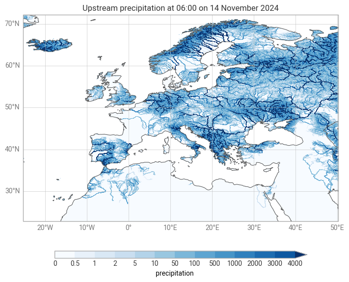

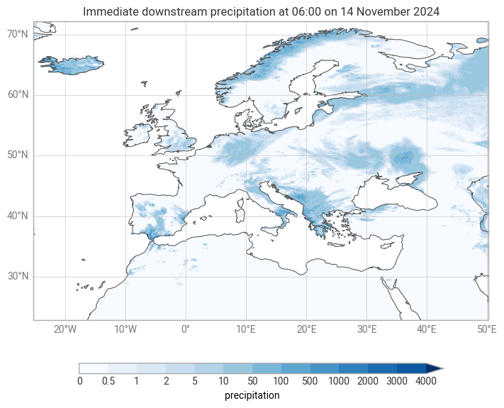
Local aggregation¶

Local aggregations can be computed using the move submodule, and the same metrics are available.

Below we show an example using move.downstream to find the number of gridcells draining to each point.

move_downstream = ekh.move.downstream(network, da, metric="sum")

chart = ekp.Map()
chart.quickplot(move_downstream, style=style)
chart.legend(label="{variable_name}")
chart.title("Immediate downstream precipitation at {time:%H:%M on %-d %B %Y}")
chart.coastlines()
chart.gridlines()
chart.show()